Show Code
import numpy as np
import torch
import torch.nn as nn

import matplotlib.pyplot as pltIn vesion 1 we trained a character-level RNN on Arabic text, but the generated text was not very coherent. We used a simple RNN architecture with one RNN layer and a fully connected output layer. In this version, we will make some improvements to the model architecture and compare the results.
But first, what is the problem with the previous model? The main issue is that a simple RNN has limited capacity to capture long-range dependencies in the text. This means that it struggles to remember information from earlier in the sequence. The question is: why it is struggling to remember?
The problem is vanishing gradient problem. During training, the gradients used to update the model’s weights can become very small as they are backpropagated through many time steps. This makes it difficult for the model to learn long-range dependencies.
import numpy as np
import torch
import torch.nn as nn
import matplotlib.pyplot as plt#importing the dataset
with open('data/arabic_text.txt', 'r', encoding='utf-8') as f:
text = f.read()
# Creating a set of unique characters in the text
print(f'Length of text: {len(text)} characters')
chars = sorted(list(set(text)))
print(f'Unique characters: {len(chars)}')
print(f'Sample characters: {chars[10:20]}')Length of text: 3296 characters
Unique characters: 47
Sample characters: ['ئ', 'ا', 'ب', 'ة', 'ت', 'ث', 'ج', 'ح', 'خ', 'د']The first step after imprting the data and taking the unique characters is to create a mapping of characters to integers and vice versa. We will create two dictionaries: char_to_int and int_to_char. The char_to_int dictionary will map each unique character to a unique integer, while the int_to_char dictionary will do the reverse mapping.
char_to_int = {char: idx for idx, char in enumerate(chars)}
int_to_char = {idx: char for idx, char in enumerate(chars)}
print(f'Character to Integer Mapping: {list(char_to_int.items())[10:20]}')
Character to Integer Mapping: [('ئ', 10), ('ا', 11), ('ب', 12), ('ة', 13), ('ت', 14), ('ث', 15), ('ج', 16), ('ح', 17), ('خ', 18), ('د', 19)]Notice how each unique character in the text is assigned a unique integer. This mapping will be used to convert the text into a format that can be fed into the RNN model for training.
seq_length = 100
dataX = []
dataY = []
for i in range(0, len(text) - seq_length):
    seq_in = text[i:i + seq_length] # the char (i + seq_length) not included in the input sequence
    seq_out = text[i + seq_length] # the char (i + seq_length) is the output character that we want to predict
    dataX.append([char_to_int[char] for char in seq_in])
    dataY.append(char_to_int[seq_out])

print(f'Total Sequences: {len(dataX)}')
print(f'Sample Input Sequence: {dataX[0]}')
print(f'Sample Output Character: {int_to_char[dataY[0]]}')
Total Sequences: 3196
Sample Input Sequence: [31, 40, 1, 11, 34, 12, 19, 11, 40, 13, 4, 1, 33, 11, 36, 14, 1, 11, 34, 7, 21, 26, 1, 18, 11, 34, 40, 13, 1, 38, 31, 11, 21, 30, 13, 4, 1, 38, 33, 11, 36, 14, 1, 11, 34, 28, 34, 35, 13, 1, 14, 29, 34, 38, 1, 38, 16, 37, 1, 11, 34, 30, 35, 21, 2, 0, 11, 34, 29, 34, 35, 1, 36, 38, 21, 1, 38, 11, 34, 16, 37, 34, 1, 28, 34, 11, 35, 4, 1, 31, 11, 27, 34, 12, 1, 11, 34, 29, 34, 35]
Sample Output Character: # Converting the data into PyTorch tensors
X = torch.tensor(dataX, dtype=torch.long)
y = torch.tensor(dataY, dtype=torch.long)
print(f'Input Tensor Shape: {X.shape}')
print(f'Output Tensor Shape: {y.shape}')Input Tensor Shape: torch.Size([3196, 100])
Output Tensor Shape: torch.Size([3196])We will define a simple RNN model using PyTorch.
## Defining the RNN Model
class CharRNN(nn.Module):
    def __init__(self, input_size, hidden_size, output_size, test=False):
        super(CharRNN, self).__init__() # Calls nn.Module's (The parent class) and own its __init__.
        self.hidden_size = hidden_size
        self.rnn = nn.RNN(input_size, hidden_size, batch_first=True) # batch_first=True --> (batch, seq_length, input_size)
        self.fc = nn.Linear(hidden_size, output_size)
        self.test = test

    def forward(self, x, hidden):
        out, hidden = self.rnn(x, hidden)
        if self.test:
            print(f'RNN output shape (before fc): {out.shape}')  # add this
            print(f'Last timestep shape (before fc): {out[:, -1, :].shape}')
        out = self.fc(out[:, -1, :])  # the output shape is (batch_size, sequence_length, hidden_size), we will take the
        # last output of the sequence and pass it through the fully connected layer to get the final output shape of (batch_size, output_size)
        return out, hidden

    def init_hidden(self, batch_size, device): # Initialize hidden state with zeros
        return torch.zeros(1, batch_size, self.hidden_size).to(device)


input_size = len(chars)
hidden_size = 256
output_size = len(chars)
model = CharRNN(input_size, hidden_size, output_size, test=True)
print(model)
CharRNN(
(rnn): RNN(47, 256, batch_first=True)
(fc): Linear(in_features=256, out_features=47, bias=True)
)# pass a sample input through the model to check the output shape
sample_input = X[0].unsqueeze(0) # Add batch dimension
sample_input = nn.functional.one_hot(sample_input, num_classes=input_size).float() # Convert to one-hot encoding
print(f'Sample Input Shape: {sample_input.shape}')
hidden = model.init_hidden(batch_size=1, device='cpu')
output, hidden = model(sample_input, hidden)
print(f'Sample Output Shape after fc, the 256 got mapped to 47: {output.shape}, These are the logits; a scalar value for each character in the vocabulary.')Sample Input Shape: torch.Size([1, 100, 47])
RNN output shape (before fc): torch.Size([1, 100, 256])
Last timestep shape (before fc): torch.Size([1, 256])
Sample Output Shape after fc, the 256 got mapped to 47: torch.Size([1, 47]), These are the logits; a scalar value for each character in the vocabulary.criterion = nn.CrossEntropyLoss()
# do one forward + backward pass
hidden = model.init_hidden(batch_size=1, device='cpu')
output, hidden = model(sample_input, hidden)
loss = criterion(output, y[0:1])
loss.backward()
# print gradient norm for each parameter
for name, param in model.named_parameters():
if param.grad is not None:
print(f"{name:30s} grad norm: {param.grad.norm().item():.6f}")RNN output shape (before fc): torch.Size([1, 100, 256])
Last timestep shape (before fc): torch.Size([1, 256])
rnn.weight_ih_l0 grad norm: 0.691554
rnn.weight_hh_l0 grad norm: 0.771839
rnn.bias_ih_l0 grad norm: 0.708893
rnn.bias_hh_l0 grad norm: 0.708893
fc.weight grad norm: 1.106892
fc.bias grad norm: 0.988741We will use the above gradinet access to see how gradients are flowing through the model during training. This can help us understand how the model is learning and whether it is suffering from the vanishing gradient problem.
The change we made to the training loop is that we are now recording the gradient norms at each training step. Using the L2 norm of the gradients, we can track how the gradients are changing over time. The p.grad.norm() already computes the L2 norm within one layer. Squaring (see ** 2) it un-does that square root so you can accumulate raw sums of squares across all layers. Then the final ** 0.5 takes one square root over everything.
The math: total_norm = √( ‖layer0_grads‖² + ‖layer1_grads‖² + ... ) = √( Σ all_gradients² )
The norm is a single scalar value that represents the overall magnitude of the gradients across all layers.
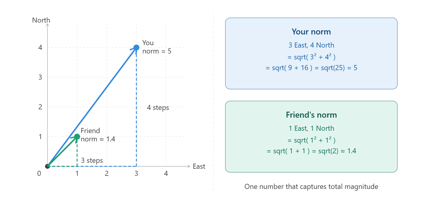
In the norm for gradients we collapse all the gradients into a single scalar value that represents the overall magnitude of the gradients across all layers.
input_size = len(chars)
hidden_size = 256
output_size = len(chars)

model = CharRNN(input_size, hidden_size, output_size)
criterion = nn.CrossEntropyLoss()
optimizer = torch.optim.Adam(model.parameters(), lr=0.001)


epochs = 100
batch_size = 64
grad_norms = []
losses = []

for epoch in range(epochs):
    model.train()
    total_loss = 0
    for i in range(0, len(X) - batch_size, batch_size): #loop through the data in batches
        X_batch = X[i:i + batch_size]
        Y_batch = y[i:i + batch_size]

        # Convert inputs to one-hot encoding
        X_batch_one_hot = nn.functional.one_hot(X_batch, num_classes=input_size).float()

        # Initialize hidden state
        hidden = model.init_hidden(batch_size, device='cpu')

        # Forward pass
        outputs, hidden = model(X_batch_one_hot, hidden)

        # Compute loss
        loss = criterion(outputs, Y_batch)

        # Backward pass and optimization
        optimizer.zero_grad()
        loss.backward()
        optimizer.step()

        # Record gradient norms
        total_norm = 0
        for p in model.parameters():
            if p.grad is not None:
                total_norm += p.grad.norm().item() ** 2 # sum of squared norms per layer
        grad_norms.append(total_norm ** 0.5) # take the square root to get the overall norm

        total_loss += loss.item()

    avg_loss = total_loss / (len(X) // batch_size)
    losses.append(avg_loss)
    print(f'Epoch [{epoch+1}/{epochs}], Loss: {avg_loss:.4f}')
Epoch [1/100], Loss: 3.2565
Epoch [2/100], Loss: 3.0947
Epoch [3/100], Loss: 2.9248
Epoch [4/100], Loss: 2.7636
Epoch [5/100], Loss: 2.6466
Epoch [6/100], Loss: 2.5711
Epoch [7/100], Loss: 2.5003
Epoch [8/100], Loss: 2.4592
Epoch [9/100], Loss: 2.4301
Epoch [10/100], Loss: 2.3847
Epoch [11/100], Loss: 2.3363
Epoch [12/100], Loss: 2.2934
Epoch [13/100], Loss: 2.2375
Epoch [14/100], Loss: 2.1825
Epoch [15/100], Loss: 2.1522
Epoch [16/100], Loss: 2.1127
Epoch [17/100], Loss: 2.0729
Epoch [18/100], Loss: 2.0197
Epoch [19/100], Loss: 1.9669
Epoch [20/100], Loss: 1.9208
Epoch [21/100], Loss: 1.8504
Epoch [22/100], Loss: 1.8422
Epoch [23/100], Loss: 1.7846
Epoch [24/100], Loss: 1.6958
Epoch [25/100], Loss: 1.6389
Epoch [26/100], Loss: 1.5922
Epoch [27/100], Loss: 1.5788
Epoch [28/100], Loss: 1.5416
Epoch [29/100], Loss: 1.4577
Epoch [30/100], Loss: 1.3991
Epoch [31/100], Loss: 1.3579
Epoch [32/100], Loss: 1.3230
Epoch [33/100], Loss: 1.2754
Epoch [34/100], Loss: 1.1785
Epoch [35/100], Loss: 1.1283
Epoch [36/100], Loss: 1.1112
Epoch [37/100], Loss: 1.0890
Epoch [38/100], Loss: 1.0959
Epoch [39/100], Loss: 1.0425
Epoch [40/100], Loss: 0.9640
Epoch [41/100], Loss: 0.8750
Epoch [42/100], Loss: 0.7882
Epoch [43/100], Loss: 0.7421
Epoch [44/100], Loss: 0.6971
Epoch [45/100], Loss: 0.6382
Epoch [46/100], Loss: 0.6035
Epoch [47/100], Loss: 0.5705
Epoch [48/100], Loss: 0.5048
Epoch [49/100], Loss: 0.4754
Epoch [50/100], Loss: 0.4230
Epoch [51/100], Loss: 0.4007
Epoch [52/100], Loss: 0.3500
Epoch [53/100], Loss: 0.3141
Epoch [54/100], Loss: 0.2881
Epoch [55/100], Loss: 0.2631
Epoch [56/100], Loss: 0.2288
Epoch [57/100], Loss: 0.1906
Epoch [58/100], Loss: 0.1634
Epoch [59/100], Loss: 0.1270
Epoch [60/100], Loss: 0.1073
Epoch [61/100], Loss: 0.0897
Epoch [62/100], Loss: 0.0735
Epoch [63/100], Loss: 0.0596
Epoch [64/100], Loss: 0.0513
Epoch [65/100], Loss: 0.0453
Epoch [66/100], Loss: 0.0408
Epoch [67/100], Loss: 0.0369
Epoch [68/100], Loss: 0.0333
Epoch [69/100], Loss: 0.0304
Epoch [70/100], Loss: 0.0280
Epoch [71/100], Loss: 0.0260
Epoch [72/100], Loss: 0.0242
Epoch [73/100], Loss: 0.0230
Epoch [74/100], Loss: 0.0219
Epoch [75/100], Loss: 0.0212
Epoch [76/100], Loss: 0.0201
Epoch [77/100], Loss: 0.0187
Epoch [78/100], Loss: 0.0174
Epoch [79/100], Loss: 0.0164
Epoch [80/100], Loss: 0.0156
Epoch [81/100], Loss: 0.0149
Epoch [82/100], Loss: 0.0144
Epoch [83/100], Loss: 0.0139
Epoch [84/100], Loss: 0.0135
Epoch [85/100], Loss: 0.0130
Epoch [86/100], Loss: 0.0125
Epoch [87/100], Loss: 0.0120
Epoch [88/100], Loss: 0.0114
Epoch [89/100], Loss: 0.0111
Epoch [90/100], Loss: 0.0107
Epoch [91/100], Loss: 0.0102
Epoch [92/100], Loss: 0.0098
Epoch [93/100], Loss: 0.0101
Epoch [94/100], Loss: 0.0104
Epoch [95/100], Loss: 0.0104
Epoch [96/100], Loss: 0.0105
Epoch [97/100], Loss: 0.0118
Epoch [98/100], Loss: 0.0258
Epoch [99/100], Loss: 3.2458
Epoch [100/100], Loss: 2.8207plt.plot(losses[:-3]) # Plotting the loss over epochs, excluding the last 3 points to focus on the earlier part of training
plt.title("Training Loss over Epochs")
plt.xlabel("Epoch")
plt.ylabel("Loss")
plt.show()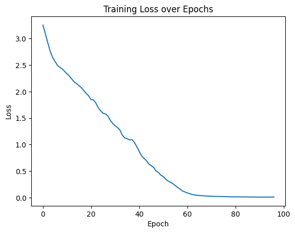
plt.plot(grad_norms[:-150])
plt.title("Gradient norm over training")
plt.xlabel("Iteration")
plt.ylabel("Gradient norm")
plt.show()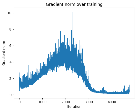
From the plot of the gradient norms, we can see 4 stages of training: 1. Initial Stage: 0 to ~1000: Model waking up, finding direction. Normal. 2. Stage 2: ~1000 to ~4000: Active learning, healthy spikes. Normal. 3. Stage 3: 2500 to ~3000: Gradients collapse from 5 to near zero. This is too sudden for natural convergence. 4. Stage 4: ~4000 to end: Gradients are near zero, model is stuck. This is a sign of vanishing gradients.
What is likely happening after epoch 2500?
The model overfit. The dataset is small, and the model has enough capacity to memorize it. After memorization, the gradients become very small because the model is not learning anything new.
In the below code, will take the trained model and generate new text based on a starting string. We will take the starting string, then predict the next 200 characters one by one, feeding the predicted character back into the model at each step.
def predict(model, start_str, predict_len=200, temperature=0.8):
    model.eval()

    # convert starting string to indices
    # pad the seed to seq_length=100
    if len(start_str) < seq_length:
        start_str = ' ' * (seq_length - len(start_str)) + start_str
    input_seq = [char_to_int[ch] for ch in start_str]
    input_tensor = torch.tensor(input_seq).unsqueeze(0)  # [1, seq_len] - Add batch dimension

    hidden = model.init_hidden(batch_size=1, device='cpu')
    generated = start_str

    for _ in range(predict_len):

        # one-hot encode for each character in the input sequence
        x = nn.functional.one_hot(input_tensor, num_classes=input_size).float()  # [1, seq_len, 47]

        # forward pass
        output, hidden = model(x, hidden)  # output: [1, 47], for what character comes next

        # apply temperature then sample
        output = output / temperature # with temperature < 1, high-probability chars get even higher
        probs = torch.softmax(output, dim=1)  # [1, 47] - convert logits to probabilities
        next_char_idx = torch.multinomial(probs, num_samples=1).item() # sample the next character index based on the probabilities

        # append predicted character
        next_char = int_to_char[next_char_idx]
        generated += next_char

        # slide the window — drop first char, append predicted
        input_seq = input_seq[1:] + [next_char_idx]
        input_tensor = torch.tensor(input_seq).unsqueeze(0)

    return generated


# run it
print(predict(model, start_str='رحلة '))
رحلة تح يس ب.
الص اميح ن لسة فب تبييحح اراتعوح الابا حابام حبقدبح با ابلا.
بالتصومح قلل يت حالاص.
التندة
الضا.
ا االش
بص صلهق شالح و بهالص اس حيوحت كبة تسيصت عوا اباصتذت ال اق.
الغي بخد توقح ومح القوحديت The main issue with the previous model was that it was trained on a very small dataset, which made it easy for the model to overfit and memorize the training data. To address this issue, we will train the model on a larger dataset of Arabic text.
# Load the pre-downloaded CALM/arwiki slice (10k articles, ~1.6M chars).
with open('../../../rnn/data/arwiki_10k.txt', 'r', encoding='utf-8') as f:
    text = f.read()

print(f'Length of text: {len(text):,} characters')
Length of text: 1,660,735 characters# process the new dataset
chars = sorted(list(set(text)))
vocab_size = len(chars)
print(f'Unique characters: {vocab_size}')
char_to_int = {char: idx for idx, char in enumerate(chars)}
int_to_char = {idx: char for idx, char in enumerate(chars)}
# create training sequences
seq_length = 100
dataX = []
dataY = []
for i in range(0, len(text) - seq_length, seq_length):
seq_in = text[i:i + seq_length]
seq_out = text[i + seq_length]
dataX.append([char_to_int[char] for char in seq_in])
dataY.append(char_to_int[seq_out])
print(f'Total Sequences: {len(dataX):,}')
print(f'Sample Input Sequence: {dataX[0]}')
# Convert to tensors
X = torch.tensor(dataX, dtype=torch.long)
y = torch.tensor(dataY, dtype=torch.long)
print(f'Input Tensor Shape: {X.shape}')
print(f'Output Tensor Shape: {y.shape}')
Unique characters: 458
Total Sequences: 16,607
Sample Input Sequence: [280, 290, 260, 255, 282, 291, 263, 1, 256, 293, 281, 1, 260, 289, 256, 293, 265, 1, 9, 283, 285, 290, 277, 255, 279, 27, 1, 260, 290, 256, 285, 265, 10, 1, 9, 19, 18, 14, 18, 17, 21, 1, 282, 275, 1, 14, 1, 23, 21, 19, 14, 24, 19, 19, 280, 10, 1, 280, 283, 279, 284, 1, 255, 279, 267, 255, 254, 256, 1, 256, 281, 1, 251, 256, 285, 1, 255, 279, 267, 255, 254, 256, 1, 255, 279, 280, 262, 266, 283, 280, 285, 1, 255, 279, 277, 265, 268, 285, 15, 1]
Input Tensor Shape: torch.Size([16607, 100])
Output Tensor Shape: torch.Size([16607])# Training on the larger dataset
input_size = vocab_size
hidden_size = 256
output_size = vocab_size
model = CharRNN(input_size, hidden_size, output_size)
criterion = nn.CrossEntropyLoss()
optimizer = torch.optim.Adam(model.parameters(), lr=0.001)
epochs = 20
batch_size = 64
grad_norms = []
losses = []
for epoch in range(epochs):
model.train()
total_loss = 0
for i in range(0, len(X) - batch_size, batch_size):
X_batch = X[i:i + batch_size]
Y_batch = y[i:i + batch_size]
X_batch_one_hot = nn.functional.one_hot(X_batch, num_classes=input_size).float()
hidden = model.init_hidden(batch_size, device='cpu')
outputs, hidden = model(X_batch_one_hot, hidden)
loss = criterion(outputs, Y_batch)
optimizer.zero_grad()
loss.backward()
optimizer.step()
total_norm = 0
for p in model.parameters():
if p.grad is not None:
total_norm += p.grad.norm().item() ** 2
grad_norms.append(total_norm ** 0.5)
total_loss += loss.item()
avg_loss = total_loss / (len(X) // batch_size)
losses.append(avg_loss)
print(f'Epoch [{epoch+1}/{epochs}], Loss: {avg_loss:.4f}')Epoch [1/20], Loss: 3.4110
Epoch [2/20], Loss: 3.1315
Epoch [3/20], Loss: 2.9406
Epoch [4/20], Loss: 2.8197
Epoch [5/20], Loss: 2.6938
Epoch [6/20], Loss: 2.5925
Epoch [7/20], Loss: 2.5193
Epoch [8/20], Loss: 2.4575
Epoch [9/20], Loss: 2.4023
Epoch [10/20], Loss: 2.3492
Epoch [11/20], Loss: 2.2980
Epoch [12/20], Loss: 2.2469
Epoch [13/20], Loss: 2.2042
Epoch [14/20], Loss: 2.1593
Epoch [15/20], Loss: 2.1145
Epoch [16/20], Loss: 2.0761
Epoch [17/20], Loss: 2.0492
Epoch [18/20], Loss: 2.0110
Epoch [19/20], Loss: 1.9807
Epoch [20/20], Loss: 1.9466plt.plot(grad_norms)
plt.title("Gradient norm over training")
plt.xlabel("Iteration")
plt.ylabel("Gradient norm")
plt.show()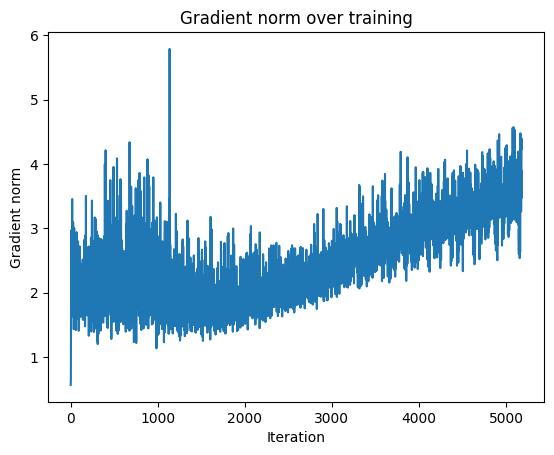
def predict(model, start_str, predict_len=200, temperature=0.2):
    model.eval()

    # convert starting string to indices
    # pad the seed to seq_length=100
    if len(start_str) < seq_length:
        start_str = ' ' * (seq_length - len(start_str)) + start_str
    input_seq = [char_to_int[ch] for ch in start_str]
    input_tensor = torch.tensor(input_seq).unsqueeze(
        0)  # [1, seq_len] - Add batch dimension

    hidden = model.init_hidden(batch_size=1, device='cpu')
    generated = start_str

    for _ in range(predict_len):

        # one-hot encode for each character in the input sequence
        x = nn.functional.one_hot(
            input_tensor, num_classes=input_size).float()  # [1, seq_len, 47]

        # forward pass
        # output: [1, 47], for what character comes next
        output, hidden = model(x, hidden)

        # apply temperature then sample
        # with temperature < 1, high-probability chars get even higher
        output = output / temperature
        # [1, 47] - convert logits to probabilities
        probs = torch.softmax(output, dim=1)
        # sample the next character index based on the probabilities
        next_char_idx = torch.multinomial(probs, num_samples=1).item()

        # append predicted character
        next_char = int_to_char[next_char_idx]
        generated += next_char

        # slide the window — drop first char, append predicted
        input_seq = input_seq[1:] + [next_char_idx]
        input_tensor = torch.tensor(input_seq).unsqueeze(0)

    return generated


# run it
print(predict(model, start_str='فأصبحت تعرف منذ ذلك العهد'))
فأصبحت تعرف منذ ذلك العهد معادم المنسي السمامي الأملال المي مالسي من المنسم الميلمينتي قلى المن التم يقع لمعال عام 1978 وي كارب السم العدمث المالي السم العمام المي من المنسم المولية المستي المت في المناد المالم السم العملم ال
Comments