Show Code
import torch
import torch.nn as nn
import torch.optim as optim
from torchvision import datasets, transformsIn this notebook we will try implementing the first version LeNet archetecture, then see the results and try matching it with the orignal authors’ results, then implement different approaches to see the effect of a change in the network.
import torch
import torch.nn as nn
import torch.optim as optim
from torchvision import datasets, transformsThe LeNet uses MNIST dataset which is a collection of hand written digits.
# Define transformations for the MNIST dataset
transform = transforms.Compose([
    transforms.Resize((28, 28)),   # LeNet expects 28x28 input images
    transforms.ToTensor(),
    transforms.Normalize((0.1307,), (0.3081,))
])

# Load MNIST dataset for training
train_dataset = datasets.MNIST(
    root="./data",
    train=True,
    download=True,
    transform=transform
)
# Load test dataset
test_dataset = datasets.MNIST(
    root="./data",
    train=False,
    transform=transform
)
# Create data loaders that will handle batching and shuffling
train_loader = torch.utils.data.DataLoader(
    train_dataset, batch_size=32, shuffle=True
)

test_loader = torch.utils.data.DataLoader(
    test_dataset, batch_size=1000, shuffle=False
)
0.3%0.7%1.0%1.3%1.7%2.0%2.3%2.6%3.0%3.3%3.6%4.0%4.3%4.6%5.0%5.3%5.6%6.0%6.3%6.6%6.9%7.3%7.6%7.9%8.3%8.6%8.9%9.3%9.6%9.9%10.2%10.6%10.9%11.2%11.6%11.9%12.2%12.6%12.9%13.2%13.6%13.9%14.2%14.5%14.9%15.2%15.5%15.9%16.2%16.5%16.9%17.2%17.5%17.9%18.2%18.5%18.8%19.2%19.5%19.8%20.2%20.5%20.8%21.2%21.5%21.8%22.1%22.5%22.8%23.1%23.5%23.8%24.1%24.5%24.8%25.1%25.5%25.8%26.1%26.4%26.8%27.1%27.4%27.8%28.1%28.4%28.8%29.1%29.4%29.8%30.1%30.4%30.7%31.1%31.4%31.7%32.1%32.4%32.7%33.1%33.4%33.7%34.0%34.4%34.7%35.0%35.4%35.7%36.0%36.4%36.7%37.0%37.4%37.7%38.0%38.3%38.7%39.0%39.3%39.7%40.0%40.3%40.7%41.0%41.3%41.7%42.0%42.3%42.6%43.0%43.3%43.6%44.0%44.3%44.6%45.0%45.3%45.6%45.9%46.3%46.6%46.9%47.3%47.6%47.9%48.3%48.6%48.9%49.3%49.6%49.9%50.2%50.6%50.9%51.2%51.6%51.9%52.2%52.6%52.9%53.2%53.6%53.9%54.2%54.5%54.9%55.2%55.5%55.9%56.2%56.5%56.9%57.2%57.5%57.9%58.2%58.5%58.8%59.2%59.5%59.8%60.2%60.5%60.8%61.2%61.5%61.8%62.1%62.5%62.8%63.1%63.5%63.8%64.1%64.5%64.8%65.1%65.5%65.8%66.1%66.4%66.8%67.1%67.4%67.8%68.1%68.4%68.8%69.1%69.4%69.8%70.1%70.4%70.7%71.1%71.4%71.7%72.1%72.4%72.7%73.1%73.4%73.7%74.0%74.4%74.7%75.0%75.4%75.7%76.0%76.4%76.7%77.0%77.4%77.7%78.0%78.3%78.7%79.0%79.3%79.7%80.0%80.3%80.7%81.0%81.3%81.7%82.0%82.3%82.6%83.0%83.3%83.6%84.0%84.3%84.6%85.0%85.3%85.6%85.9%86.3%86.6%86.9%87.3%87.6%87.9%88.3%88.6%88.9%89.3%89.6%89.9%90.2%90.6%90.9%91.2%91.6%91.9%92.2%92.6%92.9%93.2%93.6%93.9%94.2%94.5%94.9%95.2%95.5%95.9%96.2%96.5%96.9%97.2%97.5%97.9%98.2%98.5%98.8%99.2%99.5%99.8%100.0%
100.0%
2.0%4.0%6.0%7.9%9.9%11.9%13.9%15.9%17.9%19.9%21.9%23.8%25.8%27.8%29.8%31.8%33.8%35.8%37.8%39.7%41.7%43.7%45.7%47.7%49.7%51.7%53.7%55.6%57.6%59.6%61.6%63.6%65.6%67.6%69.6%71.5%73.5%75.5%77.5%79.5%81.5%83.5%85.5%87.4%89.4%91.4%93.4%95.4%97.4%99.4%100.0%
100.0%class LeNet1(nn.Module):
def __init__(self):
super().__init__()
# C1
self.conv1 = nn.Conv2d(1, 4, kernel_size=5) # 4 feature maps
# S1
self.pool1 = nn.AvgPool2d(2, 2)
# C2
self.conv2 = nn.Conv2d(4, 8, kernel_size=5) # 8 feature maps
# S2
self.pool2 = nn.AvgPool2d(2, 2)
# FC
self.fc = nn.Linear(8 * 4 * 4, 10)
self.activation = torch.tanh
def forward(self, x):
x = self.activation(self.conv1(x)) # 28→24
x = self.pool1(x) # 24→12
x = self.activation(self.conv2(x)) # 12→8
x = self.pool2(x) # 8→4
x = x.view(x.size(0), -1) # 8×4×4 #x.size(0) keeps the batch size and -1 flattens the rest (N, 8*4*4) → (N, 128)
x = self.fc(x)
return xdevice = torch.device("cuda" if torch.cuda.is_available() else "cpu")
model = LeNet1().to(device)
criterion = nn.CrossEntropyLoss()
#criterion = nn.MSELoss()
optimizer = optim.SGD(
model.parameters(),
lr=0.01,
momentum=0.9
)def train(model, device, train_loader, optimizer, criterion, epoch):
# Set model to training mode
model.train()
running_loss = 0.0
correct = 0
total = 0
for batch_idx, (data, target) in enumerate(train_loader):
# Move data to the appropriate device
data, target = data.to(device), target.to(device)
# Zero the gradients
optimizer.zero_grad()
# Forward pass
output = model(data)
# Compute loss
loss = criterion(output, target)
# Backward pass and optimization
loss.backward()
optimizer.step()
# Accumulate loss
running_loss += loss.item() * data.size(0)
# Accumulate accuracy
pred = output.argmax(dim=1)
correct += (pred == target).sum().item()
total += target.size(0)
avg_loss = running_loss / total
accuracy = correct / total
print(
f"Epoch {epoch}:"
f" Avg Loss: {avg_loss:.4f}, Accuracy: {accuracy:.4f}"
)
return avg_loss, accuracyBelow, .sum() counts the number of True values (i.e., correct predictions) in the batch. .item() converts this count from a tensor to a Python number.
target.size(0) gives the number of samples in the current batch.def test(model, device, test_loader):
# Set model to evaluation mode
model.eval()
# Initialize counters
correct = 0
total = 0
with torch.no_grad():
for data, target in test_loader:
data, target = data.to(device), target.to(device)
# Forward pass
output = model(data)
# Get predictions
pred = output.argmax(dim=1)
# Update counters
correct += (pred == target).sum().item()
total += target.size(0)
accuracy = correct / total
return accuracytrain_losses = []
train_accuracies = []
test_accuracies = []
for epoch in range(1, 20):
train_loss, train_acc = train(model, device, train_loader, optimizer, criterion, epoch)
test_acc = test(model, device, test_loader)
train_losses.append(train_loss)
train_accuracies.append(train_acc)
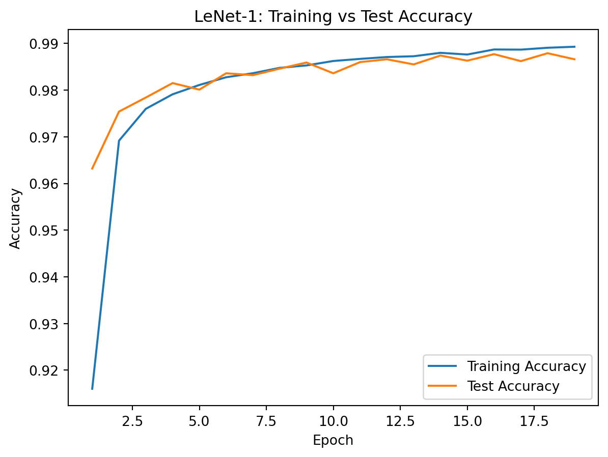
test_accuracies.append(test_acc)Epoch 1: Avg Loss: 0.2980, Accuracy: 0.9160
Epoch 2: Avg Loss: 0.1074, Accuracy: 0.9692
Epoch 3: Avg Loss: 0.0830, Accuracy: 0.9760
Epoch 4: Avg Loss: 0.0710, Accuracy: 0.9791
Epoch 5: Avg Loss: 0.0637, Accuracy: 0.9811
Epoch 6: Avg Loss: 0.0581, Accuracy: 0.9828
Epoch 7: Avg Loss: 0.0546, Accuracy: 0.9836
Epoch 8: Avg Loss: 0.0513, Accuracy: 0.9848
Epoch 9: Avg Loss: 0.0488, Accuracy: 0.9853
Epoch 10: Avg Loss: 0.0467, Accuracy: 0.9862
Epoch 11: Avg Loss: 0.0448, Accuracy: 0.9867
Epoch 12: Avg Loss: 0.0435, Accuracy: 0.9871
Epoch 13: Avg Loss: 0.0424, Accuracy: 0.9872
Epoch 14: Avg Loss: 0.0407, Accuracy: 0.9880
Epoch 15: Avg Loss: 0.0405, Accuracy: 0.9876
Epoch 16: Avg Loss: 0.0388, Accuracy: 0.9887
Epoch 17: Avg Loss: 0.0380, Accuracy: 0.9887
Epoch 18: Avg Loss: 0.0370, Accuracy: 0.9891
Epoch 19: Avg Loss: 0.0361, Accuracy: 0.9893import matplotlib.pyplot as plt
epochs = range(1, len(train_accuracies) + 1)
plt.figure()
plt.plot(train_losses)
plt.xlabel("Epoch")
plt.ylabel("Loss")
plt.title("Training Loss Drop (LeNet-1)")
plt.show()
plt.figure()
plt.plot(epochs, train_accuracies, label="Training Accuracy")
plt.plot(epochs, test_accuracies, label="Test Accuracy")
plt.xlabel("Epoch")
plt.ylabel("Accuracy")
plt.title("LeNet-1: Training vs Test Accuracy")
plt.legend()
plt.show()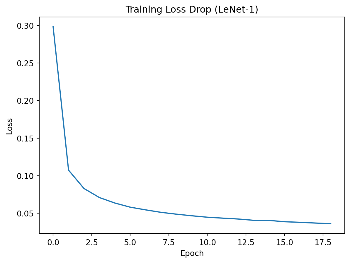
print(f"Final Training Loss: {train_losses[-1]:.4f}")
print(f"Final Training Accuracy: {train_accuracies[-1] * 100:.2f}%")
Final Training Loss: 0.0361
Final Training Accuracy: 98.93%# After training loop
print(f"Final Test Accuracy: {test_accuracies[-1]:.4f}")
print(f"Final Test Error Rate: {(1 - test_accuracies[-1]) * 100:.2f}%")Final Test Accuracy: 0.9866
Final Test Error Rate: 1.34%
Comments