Show Code
#import libraries
import torch
import torch.nn as nn
from torchviz import make_dot
from torchvision import datasets, transforms
from torch.utils.data import DataLoader


import numpy as np
import matplotlib.pyplot as pltWe will use pytorch to build a simple convolutional neural network (CNN) and break down its components step by step, and see how it trains on PyTorch. We will use the MNIST dataset, which consists of 28x28 grayscale images of handwritten digits (0-9).
#import libraries
import torch
import torch.nn as nn
from torchviz import make_dot
from torchvision import datasets, transforms
from torch.utils.data import DataLoader
import numpy as np
import matplotlib.pyplot as pltWe will start by defining the dataset and data loaders for training and testing. We will use the torchvision library to load the MNIST dataset.
# import data

train_data = datasets.MNIST(root='data', train=True, download=True, transform=transforms.ToTensor())
test_data = datasets.MNIST(root='data', train=False, download=True, transform=transforms.ToTensor())
train_loader = DataLoader(train_data, batch_size=64, shuffle=True)
test_loader = DataLoader(test_data, batch_size=64, shuffle=False)# plot some samples
examples = enumerate(train_loader) # this will give us an iterator that returns (batch_idx, (example_data, example_targets))
batch_idx, (example_data, example_targets) = next(examples) # this will give us the first batch of data and targets
fig = plt.figure()
for i in range(6):
plt.subplot(2, 3, i + 1)
plt.tight_layout()
plt.imshow(example_data[i][0], cmap='gray', interpolation='none')
plt.title("Ground Truth: {}".format(example_targets[i]))
plt.xticks([])
plt.yticks([])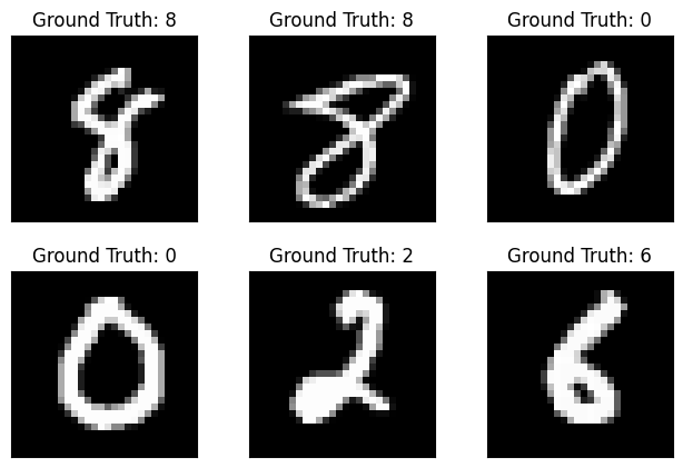
We will define a simple CNN architecture.
model = nn.Sequential(
    nn.Conv2d(1, 8, kernel_size=3, stride=1, padding=1), # input channels, output channels, kernel size
    nn.ReLU(),
    nn.Conv2d(8, 16, kernel_size=3, stride=1, padding=1),
    nn.ReLU(),
    nn.MaxPool2d(kernel_size=2, stride=2),
    nn.ReLU(),
    nn.Flatten(),
    nn.Linear(16 * 14 * 14, 32), # input features, output features
    nn.ReLU(),
    nn.Linear(32, 10) # input features, output features
)# for debugging only, print the shape of the output of each layer
x = example_data[0].unsqueeze(0) # add batch dimension
print ('Input shape:\t', x.shape)
for layer in model:
x = layer(x)
print(layer.__class__.__name__, 'output shape:\t', x.shape)
Input shape:     torch.Size([1, 1, 28, 28])
Conv2d output shape:     torch.Size([1, 8, 28, 28])
ReLU output shape:   torch.Size([1, 8, 28, 28])
Conv2d output shape:     torch.Size([1, 16, 28, 28])
ReLU output shape:   torch.Size([1, 16, 28, 28])
MaxPool2d output shape:  torch.Size([1, 16, 14, 14])
ReLU output shape:   torch.Size([1, 16, 14, 14])
Flatten output shape:    torch.Size([1, 3136])
Linear output shape:     torch.Size([1, 32])
ReLU output shape:   torch.Size([1, 32])
Linear output shape: torch.Size([1, 10])# train the model
criterion = nn.CrossEntropyLoss() # this will compute the cross-entropy loss between the predicted and true labels
optimizer = torch.optim.Adam(model.parameters(), lr=0.001) # this will optimize the
# model parameters using the Adam optimizer with a learning rate of 0.001
num_epochs = 5
for epoch in range(num_epochs):
for batch_idx, (data, targets) in enumerate(train_loader):
# forward pass
outputs = model(data)
loss = criterion(outputs, targets)
# backward pass and optimization
optimizer.zero_grad() # this will zero the gradients of the model parameters
loss.backward() # this will compute the gradients of the loss with respect to the model parameters
optimizer.step() # this will update the model parameters using the computed gradients
print(f'Epoch [{epoch+1}/{num_epochs}], Loss: {loss.item():.4f}')Epoch [1/5], Loss: 0.0403
Epoch [2/5], Loss: 0.0597
Epoch [3/5], Loss: 0.0103
Epoch [4/5], Loss: 0.0018
Epoch [5/5], Loss: 0.0061We are passing a batch of 64 images through the model on each epoch, this means: - The input to the model is of shape (64, 1, 28, 28) (batch size, channels, height, width) - Input to second layer is of shape (64, 8, 28, 28) - Input to third layer is of shape (64, 16, 28, 28) - Input to fourth layer is of shape (64, 16*14*14) (after max pooling) - Input to fifth layer is of shape (64, 32) - Input to sixth layer is of shape (64, 10) (after linear layer)
Notice that the model is working on each epoch with a batch of 64 images, this helps in making the gradient estimate more stable and less noisy compared to using a single sample.
example_data[0].unsqueeze(0).shapetorch.Size([1, 1, 28, 28])In the below code: - we took the first image from the batch - passed it through the first layer of the model, which is a Conv2d layer, outputting 8 feature maps of size 28x28 - Then plot the output, which are the 8 feature maps.
x = example_data[0].unsqueeze(0) # take only 1 example
x = model[0](x) # pass it through the first layer of the model, which is a Conv2d layer
fig, axes = plt.subplots(2, 4, figsize=(5, 3))
for i, ax in enumerate(axes.flat):
    ax.imshow(x[0][i].detach().numpy(), cmap='gray')
    ax.axis('off')
plt.suptitle(model[0].__class__.__name__)
plt.show()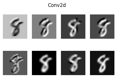
# now take those feature maps and pass them through the next layer, which is another Conv2d layer
x = model[1](x)
fig, axes = plt.subplots(2, 4, figsize=(6, 5))
for i, ax in enumerate(axes.flat):
    ax.imshow(x[0][i].detach().numpy(), cmap='gray')
    ax.axis('off')
plt.suptitle(model[1].__class__.__name__)
plt.show()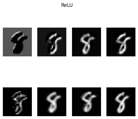
We can ask this: Why do see the number appearing in different shapes and colors in each feature map?
The different shapes and colors in each feature map represent the different features that the convolutional layer has learned to detect. Each filter in the convolutional layer is designed to detect a specific pattern or feature in the input image, such as edges, corners, or textures.
When an image is passed through the convolutional layer, each filter produces a feature map that highlights the presence of the specific feature it is designed to detect. This is the kernel_size parameter we defined in the Conv2d layer, it determines the size of the filter that is applied to the input image.
kernel_size=3 means that the filter will be a 3x3 matrix that will slide over the input image and perform convolution operations to produce the feature maps.stride=1 means that the filter will move one pixel at a time across the input image.padding=1 means that we will add a border of 1 pixel around the input image, which helps to preserve the spatial dimensions of the output feature maps.# now take those feature maps and pass them through the next layer, which is a MaxPool2d layer
x = model[2](x)
fig, axes = plt.subplots(4, 4, figsize=(6, 5))
for i, ax in enumerate(axes.flat):
ax.imshow(x[0][i].detach().numpy(), cmap='gray')
ax.axis('off')
plt.suptitle(model[2].__class__.__name__)
plt.show()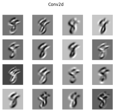
The max pooling layer reduces the spatial dimensions of the feature maps, meaning that the output feature maps will be smaller in size compared to the input feature maps, instead of 28x28 (more detailed), it will be 14x14 (less detailed) for faster computation. How this is happing in math ?
From each 2x2 block of the input feature map, the max pooling layer will take the maximum value and discard the rest. Retaining only the most important features while reducing the spatial dimensions.
We can can implement the training loop to track the gradient updates throught the backward pass, and see how the weights are updated during training.
# train the model
criterion = nn.CrossEntropyLoss()
optimizer = torch.optim.Adam(model.parameters(), lr=0.01)
num_epochs = 5
for epoch in range(num_epochs):
    for batch_idx, (data, targets) in enumerate(train_loader):
        # forward pass
        outputs = model(data)
        loss = criterion(outputs, targets)

        # backward pass and optimization
        optimizer.zero_grad()
        loss.backward()
        #inspect the gradents
        old_params = {}
        grad_params = {}
        for name, param in model.named_parameters():
            if param.grad is not None:
                old_params[name] = param.data.clone()
                grad_params[name] = param.grad.abs().mean().item()

        optimizer.step()
        #inspect the updated parameters
        delta_params = {}
        for name, param in model.named_parameters():
            if param.grad is not None:
                delta = (param.data - old_params[name]).abs().mean()
                delta_params[name] = delta.item()


    print(f'Epoch [{epoch+1}/{num_epochs}], Loss: {loss.item():.4f}')
Epoch [1/5], Loss: 0.0019
Epoch [2/5], Loss: 0.0248
Epoch [3/5], Loss: 0.0632
Epoch [4/5], Loss: 0.0589
Epoch [5/5], Loss: 0.0000
The below graph shows the average gradient updates for each layer in the network.
names = list(delta_params.keys())
values = list(delta_params.values())

plt.figure()
plt.bar(range(len(values)), values)
plt.xticks(range(len(values)), names, rotation=45, ha='right')
plt.title("Parameter Update Magnitude per Layer")
plt.ylabel("Avg |ΔW|")
plt.xlabel("Layer")
plt.tight_layout()
plt.show()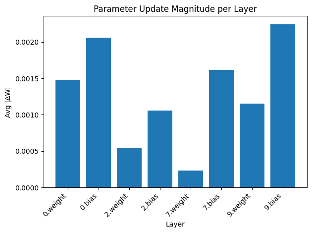
filters = model[0].weight.data  # shape: (8, 1, 3, 3)

fig, axes = plt.subplots(2, 4, figsize=(8, 4))
for i, ax in enumerate(axes.flat):
    kernel = filters[i, 0].numpy()  # shape: (3, 3)
    # normalize to [0, 1] for display
    kernel = (kernel - kernel.min()) / (kernel.max() - kernel.min() + 1e-8)
    ax.imshow(kernel, cmap='gray', interpolation='nearest')
    ax.set_title(f'Filter {i}', fontsize=9)
    ax.axis('off')

plt.suptitle('Learned Conv1 Filters (3×3)', fontsize=12)
plt.tight_layout()
plt.show()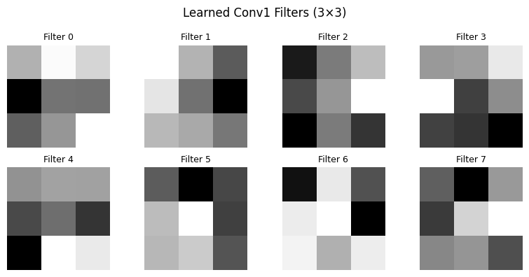
The above filters represent the learned features after the first conv layer, each filter is learning a feature (edge, or a curve, …) in the input image.
Comments