Multi Channel Convolutional Neural Networks with PyTorch

In this notebook, we will implement a simple convolutional neural network (CNN) using PyTorch to invistigate how multi-channel convolutional layers work and how data flows through the network.

IMports and data loading

# import libraries
import torch
import torch.nn as nn
from torchvision import datasets, transforms
from torch.utils.data import DataLoader
from matplotlib import pyplot as plt

transform = transforms.ToTensor()

train_data = datasets.CIFAR10(root='data', train=True, download=True, transform=transform)
test_data  = datasets.CIFAR10(root='data', train=False, download=True, transform=transform)

train_loader = DataLoader(train_data, batch_size=64, shuffle=True)
test_loader  = DataLoader(test_data,  batch_size=64, shuffle=False)

# verify shape — should be (64, 3, 32, 32)
batch, labels = next(iter(train_loader))
print(batch.shape)   # torch.Size([64, 3, 32, 32])

100.0%

torch.Size([64, 3, 32, 32])

classes = ['airplane', 'automobile', 'bird', 'cat', 'deer',
           'dog', 'frog', 'horse', 'ship', 'truck']

batch, labels = next(iter(train_loader))

fig, axes = plt.subplots(1, 4, figsize=(10, 3))
for i, ax in enumerate(axes):
    img = batch[i].permute(1, 2, 0).numpy()  # (C, H, W) → (H, W, C) for matplotlib
    ax.imshow(img)
    ax.set_title(classes[labels[i]])
    ax.axis('off')

plt.tight_layout()
plt.show()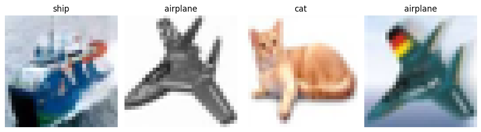

Define Model

We will define a simple CNN with two convolutional layers, followed by a fully connected layer. The first convolutional layer will have 8 filters, and the second convolutional layer will have 16 filters.

model = nn.Sequential(
    nn.Conv2d(3, 8, kernel_size=3, stride=1, padding=1),  # (3, 32, 32) → (8, 32, 32)
    nn.ReLU(),
    nn.Conv2d(8, 16, kernel_size=3, stride=1, padding=1), # (8, 32, 32) → (16, 32, 32)
    nn.ReLU(),
    nn.MaxPool2d(kernel_size=2, stride=2),                 # (16, 32, 32) → (16, 16, 16)
    nn.Flatten(),                                          # → (16 * 16 * 16) = 4096
    nn.Linear(16 * 16 * 16, 64),
    nn.ReLU(),
    nn.Linear(64, 10)
)

Pass one image through the network and inspect the output of each layer.

x = batch[0].unsqueeze(0)  # (1, 3, 32, 32)
for layer in model:
    x = layer(x)
    print(layer.__class__.__name__, x.shape)

Conv2d torch.Size([1, 8, 32, 32])
ReLU torch.Size([1, 8, 32, 32])
Conv2d torch.Size([1, 16, 32, 32])
ReLU torch.Size([1, 16, 32, 32])
MaxPool2d torch.Size([1, 16, 16, 16])
Flatten torch.Size([1, 4096])
Linear torch.Size([1, 64])
ReLU torch.Size([1, 64])
Linear torch.Size([1, 10])

Below we will manually compute the output of the first convolutional layer for the first filter, and compare it to the output produced by the layer itself. This will help us understand how multi-channel convolution works internally.

We want from the below code to understand how the convolutional layer deals with multiple input channels. We will see that the layer applies a separate kernel to each input channel, then sums the results together (plus a bias) to produce the final output for that filter.

x = batch[0].unsqueeze(0)  # (1, 3, 32, 32) — take one image

# get the learned weights for filter 0
w = model[0].weight.data  # (8, 3, 3, 3) - 8 filters produced after the first conv layer
filter0 = w[0]            # (3, 3, 3) — Take one filter, it contains 3 kernels
bias0 = model[0].bias.data[0]  # scalar, one per output channel

# manually apply each kernel to its channel
import torch.nn.functional as F

r_out = F.conv2d(x[:, 0:1, :, :], filter0[0:1].unsqueeze(0), padding=1)  # red channel
g_out = F.conv2d(x[:, 1:2, :, :], filter0[1:2].unsqueeze(0), padding=1)  # green channel
b_out = F.conv2d(x[:, 2:3, :, :], filter0[2:3].unsqueeze(0), padding=1)  # blue channel

# the summation — this is what Conv2d does internally
combined = r_out + g_out + b_out + bias0  # (1, 1, 32, 32)

# compare to what the layer actually outputs for filter 0
layer_out = model[0](x)           # (1, 8, 32, 32)
filter0_out = layer_out[:, 0:1, :, :]  # (1, 1, 32, 32)

print(torch.allclose(combined, filter0_out, atol=1e-5))  # should print True

True

Each filter contains a 3x3 kernel so we applied a convolution operation on each of the 3 channels (red, green, blue) :

Red: x[:, 0:1, :, :]

Green: x[:, 1:2, :, :]

Blue: x[:, 2:3, :, :]

with the corresponding kernels filter0[0:1], filter0[1:2], filter0[2:3]. Then sum the results together along with the bias to get the final output for that filter.

This is only for the first filter, the outout after the summation is a single channel (1, 1, 32, 32) which is the output of the first filter. The same process is repeated for each of the 8 filters in the first convolutional layer to produce an output of shape (1, 8, 32, 32). And this matches the output of the layer when we pass the image through it.

fig, axes = plt.subplots(1, 4, figsize=(12, 3))
titles = ['R contribution', 'G contribution', 'B contribution', 'Summed (filter 0 output)']
maps = [r_out, g_out, b_out, combined]

for ax, m, title in zip(axes, maps, titles):
    ax.imshow(m[0, 0].detach().numpy(), cmap='gray')
    ax.set_title(title)
    ax.axis('off')

plt.tight_layout()
plt.show()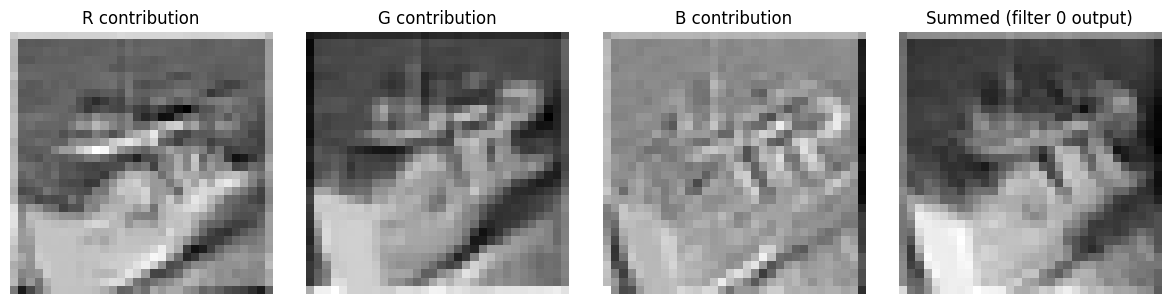

Experiment: Adding the channels first and then applying the convolution

What if we added the channels first and then applied the convolution?

To what extent the learning would be affected? To perform this experiment and compare the results, we need first to train the above model then we will modify the forward pass to add the channels first and then apply the convolution, then retrain the model and compare the results.

# Model A — standard
model_standard = nn.Sequential(
    nn.Conv2d(3, 8, kernel_size=3, padding=1),  # learns separate R/G/B kernels
    nn.ReLU(),
    nn.Conv2d(8, 16, kernel_size=3, padding=1),
    nn.ReLU(),
    nn.MaxPool2d(2, 2),
    nn.Flatten(),
    nn.Linear(16 * 16 * 16, 64),
    nn.ReLU(),
    nn.Linear(64, 10)
)

The below model is a class where we will modify the forward pass to add the channels first and then apply the convolution. The model now accepts a (B, 1, 32, 32) the B for the batch size and the 1 for the single channel after adding the 3 channels together. The other layers remain the same, we will only modify the first convolutional layer to accept a single channel input instead of 3 channels.

# Model B — sum channels first, then convolve
class SumFirstCNN(nn.Module):
    def __init__(self):
        super().__init__()
        self.conv1 = nn.Conv2d(1, 8, kernel_size=3, padding=1)  # only 1 input channel now
        self.conv2 = nn.Conv2d(8, 16, kernel_size=3, padding=1)
        self.pool  = nn.MaxPool2d(2, 2)
        self.fc1   = nn.Linear(16 * 16 * 16, 64)
        self.fc2   = nn.Linear(64, 10)

    def forward(self, x):
        x = x.sum(dim=1, keepdim=True)  # (B, 3, 32, 32) → (B, 1, 32, 32)  ← the key line
        x = F.relu(self.conv1(x))
        x = F.relu(self.conv2(x))
        x = self.pool(x)
        x = x.flatten(1)
        x = F.relu(self.fc1(x))
        return self.fc2(x)

model_sumfirst = SumFirstCNN()

Below is the code for training the model, we will train both the original model and the modified model and record the training loss and accuracy to compare the results.

def train(model, epochs=25):
    optimizer = torch.optim.Adam(model.parameters(), lr=0.001)
    criterion = nn.CrossEntropyLoss()
    losses = []

    for epoch in range(epochs):
        epoch_loss = 0
        for data, targets in train_loader:
            optimizer.zero_grad()
            loss = criterion(model(data), targets)
            loss.backward()
            optimizer.step()
            epoch_loss += loss.item()
        losses.append(epoch_loss / len(train_loader))

    correct = 0
    with torch.no_grad():
        for data, targets in test_loader:
            preds = model(data).argmax(dim=1)
            correct += (preds == targets).sum().item()
    acc = correct / len(test_loader.dataset)

    return losses, acc

losses_standard, acc_standard = train(model_standard)
losses_sumfirst,  acc_sumfirst  = train(model_sumfirst)

epochs = range(1, len(losses_standard) + 1)

fig, axes = plt.subplots(1, 2, figsize=(12, 4))

# loss
axes[0].plot(epochs, losses_standard, label='Standard (RGB)')
axes[0].plot(epochs, losses_sumfirst,  label='Sum-first')
axes[0].set_title('Training Loss per Epoch')
axes[0].set_xlabel('Epoch')
axes[0].set_ylabel('Loss')
axes[0].legend()

# accuracy
axes[1].bar(['Standard (RGB)', 'Sum-first'], [acc_standard, acc_sumfirst])
axes[1].set_title('Test Accuracy')
axes[1].set_ylabel('Accuracy')
axes[1].set_ylim(0, 1)
for i, acc in enumerate([acc_standard, acc_sumfirst]):
    axes[1].text(i, acc + 0.01, f'{acc:.3f}', ha='center')

plt.tight_layout()
plt.show()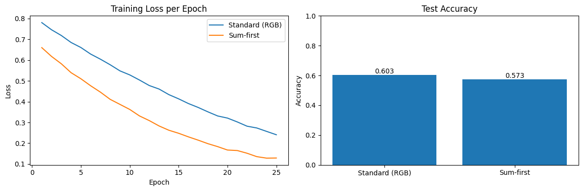

batch, labels = next(iter(train_loader))
fig, axes = plt.subplots(3, 2, figsize=(5, 8))

for i in range(3):
    img = batch[i]                                    # (3, 32, 32)
    collapsed = img.sum(dim=0, keepdim=True)          # (1, 32, 32)

    axes[i, 0].imshow(img.permute(1, 2, 0).numpy())
    axes[i, 0].set_title(f'{classes[labels[i]]} — original (RGB)')
    axes[i, 0].axis('off')

    axes[i, 1].imshow(collapsed[0].numpy(), cmap='gray')
    axes[i, 1].set_title(f'{classes[labels[i]]} — collapsed (sum)')
    axes[i, 1].axis('off')

plt.tight_layout()
plt.show()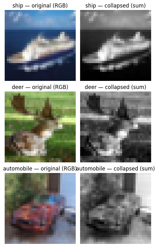

What is causing the difference in performance between the two models?

• The original model with separate kernels for each channel can learn more complex features by combining information from different channels in a more flexible way. Each filter can learn to focus on specific patterns in each channel, and then combine them to create more sophisticated features.

Recall from the previous section that each filter in the original model has 3 separate kernels (one for each channel), this is one for the red channel for example:

r_out = F.conv2d(x[:, 0:1, :, :], filter0[0:1].unsqueeze(0), padding=1)

In the above a seperate kernel is applied to the red channel, and seperate kernels are applied to the green and blue channels, thus each kernel can learn to focus on specific patterns in its respective channel. However, in the modified model we have only one kernel to the combined channels.

Next to work with:

• Compare how training in CPU vs GPU works in details.