What is an activation function?
In this explainer we will go through the concept and intuition of an activation function. Why activation functions are essential and what role they play in training AI models?
We will discuss the following:
Definition: What is an activation function?
In mathematical terms, an activation function is simply taking an input value \(x\) and transforms it into a new value. This transformation includes squashing the input into a specific range, shifting it, or introducing non-linearity. For example, some activation functions compress all inputs into the interval (0, 1), others set all negative values to zero, and some map inputs to the range (-1, 1). These different behaviors help models capture complex patterns that simple linear functions cannot.
Sigmoid activation function for example takes any input \(x\) then squashes it to a range between (0,1). This removes the linearty in the input, if the input comes from a linear relation like:
\[ w_1.x_1 + w_2.x_2 + .... + w_n.x_n \]
then the sigmoid will convert this linear combination into a non-linear output, allowing the network to learn more complex relationships.
A non-linear output means the result is not just a straight-line relationship between the input and output. The output changes in a curved way—it can bend, flatten, or squash the input values. This allows the model to learn and represent much more complex patterns.
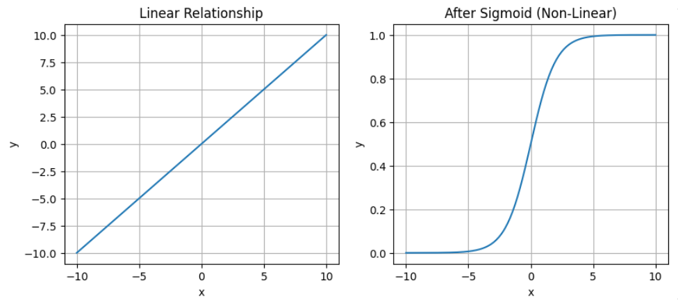 Notice how the sigmoid introduce curves and removes the linearity in line on left.
Common types: math&code
Sigmoid Function
For example: Lets take the popular activation function (Sigmoid), this function takes any input value \(x\) then map it to a range between 0 and 1:
\[ \sigma(x) = \frac{1}{1 + e^{-x}} \]
\[ \begin{aligned} x = -2 &\to \sigma(-2) \approx 0.119 \\ \\ x = -1 &\to \sigma(-1) \approx 0.269 \\ \\ x = 0 &\to \sigma(0) = 0.5\\ \\ x = 1 &\to \sigma(1) \approx 0.731 \\ \\ x = 2 &\to \sigma(2) \approx 0.881 \end{aligned} \]
From the example we see the sigmoid maps negative inputs close to 0, positive inputs close to 1, and 0 to 0.5. It squashes values into (0,1).
Consider an example where we have 200 randomly generated values, if we pass them through a sigmoid function then we get this result: 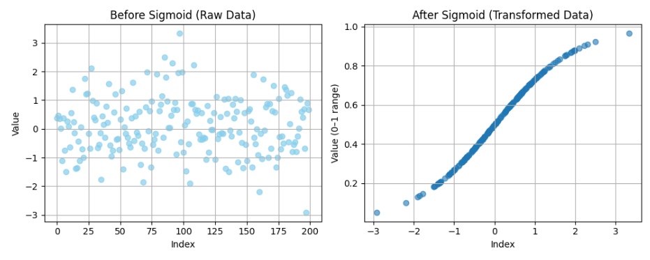
Try changing the value of \(x\) then notice the output the sigmoid function returns:
ReLU (Rectified Linear Unit)
ReLU (Rectified Linear Unit) is another popular activation function that works in a much simpler way — it keeps all positive values as they are and turns any negative value into zero: \[ \text{ReLU}(x) = \max(0, x) \]
If the input is negative, the output is 0. But if it’s positive, it passes through unchanged.
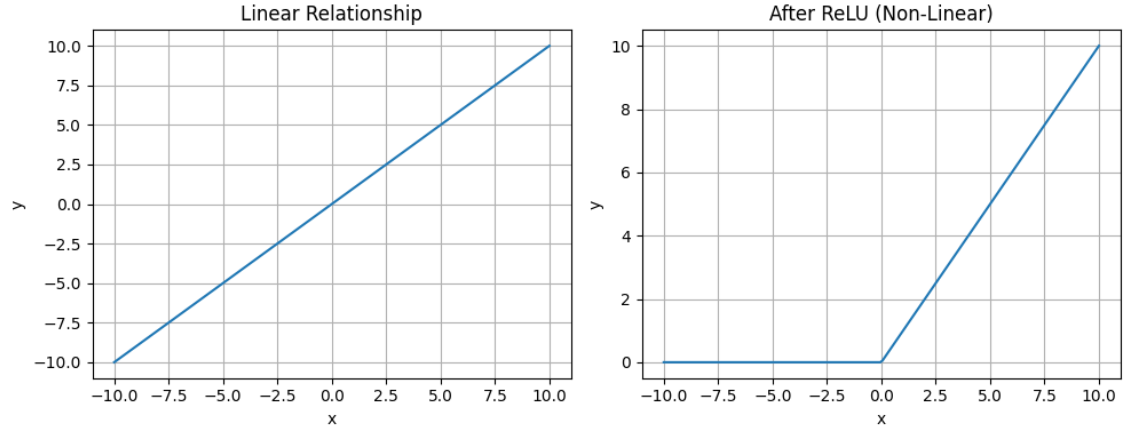
The relu function shuts off any values below 0 and turn them to 0, this effect (in model training) allows the model to ignore negative signals and only pass forward positive ones. As a result, ReLU helps neural networks learn faster and makes them more efficient, especially in deep learning.
This example shows how all values below 0 become 0 after passing through the ReLU function, while positive values remain unchanged, showing how negative inputs are filtered out and only positive values remains: 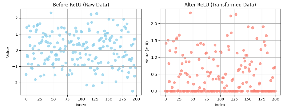
Try changing the value of \(x\) and see the retuned value from the relu function:
Try changing \(x\) to a negative value and see the result. You will notice that for any negative value you inter, the function always returns \(0\).
Softmax
The softmax activation function takes a list of input values and converts them into probabilities that sum to 1. Each output represents the probability that the input belongs to a particular class. Used commonly in the output layer of neural networks for multi-class classification problems.
For example, if you have three input values, softmax will transform them into three probabilities, and the sum of these probabilities will always be 1.
\[ \text{Softmax}(x_i) = \frac{e^{x_i}}{\sum_{j=1}^{n} e^{x_j}} \]
| Input scores | Softmax probabilities | Sum of probabilities |
|---|---|---|
| \([2.0,\ 1.0,\ 0.1]\) | \([0.659,\ 0.242,\ 0.099]\) | \(1.0\) |
The rule of the softmax function is to scale the input scores to probabilities. From the above example we see that the input score \(2.0\) has the highest probability = \(0.65\).
Try changing the numbers inside the list and see the returned value from the softmax:
Lets take the following as an example:
\[ \text{Given } \mathbf{x} = [3,\,1,\,0], \quad \text{let } m = \max(\mathbf{x}) = 3. \]
We need to subtract the maximum score \(m=max(x)\) from every element before applying the exponential, this to prevent the exponential from growing enormously large, which can cause and overflow (numbers too big for the computer to represent):
\[ \text{Shifted scores: } \mathbf{z} = \mathbf{x} - m = [0,\,-2,\,-3]. \]
This doesn’t change the result of the softmax at all — because the same constant 𝑚 is subtracted from all elements.
\[ \exp(\mathbf{z}) = [e^{0},\, e^{-2},\, e^{-3}] = [1,\, 0.1353,\, 0.0498]. \]
\[ S = \sum_j e^{z_j} = 1 + 0.1353 + 0.0498 = 1.1851. \]
\[ \mathbf{p} = \frac{\exp(\mathbf{z})}{S} = [0.8438,\, 0.1142,\, 0.0420]. \]
Summary
In this explainer we introduced activation functions and the role they play in neural networks training process. The important takeaway is that these functions introduce non-linearity makining allowing the model to learn complex patterns. We took a quick look to the most popular ones: Sigmoid, Relu, and Softmax. There are others like Tanh (similar to sigmoid), and Leaky ReLU. Each has its strengths, but ReLU and its variants are the go-to for most modern networks due to their simplicity and effectiveness. Understanding activation functions is key to building powerful neural networks, We will further explore their effects as we start building complete neural networks.
Comments