Show Code
# Run this if you're in a Colab to install MNIST 1D repository
#!pip install git+https://github.com/greydanus/mnist1dWe will explore in this example how batch normalization works and improves training stability and speed. We’ll compare a simple neural network with and without batch normalization on a small dataset, observe the effect on loss curves, and discuss the results. By the end, you’ll see how BatchNorm helps networks converge faster and generalize better.
# Run this if you're in a Colab to install MNIST 1D repository
#!pip install git+https://github.com/greydanus/mnist1dimport numpy as np
import os
import torch
import torch.nn as nn
from torch.utils.data import TensorDataset, DataLoader
from torch.optim.lr_scheduler import StepLR
import matplotlib.pyplot as plt
import mnist1d
import randomargs = mnist1d.data.get_dataset_args()
data = mnist1d.data.get_dataset(
args, path='./mnist1d_data.pkl', download=False, regenerate=False)Successfully loaded data from ./mnist1d_data.pkl# Load in the data
train_data_x = data['x'].transpose()
train_data_y = data['y']
val_data_x = data['x_test'].transpose()
val_data_y = data['y_test']def get_variance(name, data):
np_data = data.detach().numpy()
neuron_variance = np.mean(np.var(np_data, axis=0))
#print("%s variance=%f" % (name, neuron_variance))
return neuron_variance# He initialization of weights
def weights_init(layer_in):
if isinstance(layer_in, nn.Linear):
nn.init.kaiming_uniform_(layer_in.weight)
layer_in.bias.data.fill_(0.0)def train_model(model, x_train, y_train, n_epochs=20):
loss_function = nn.CrossEntropyLoss()
optimizer = torch.optim.SGD(model.parameters(), lr=0.05, momentum=0.9)
data_loader = DataLoader(TensorDataset(
x_train, y_train), batch_size=200, shuffle=True, worker_init_fn=np.random.seed(1))
# Initialize model weights once before training
model.apply(weights_init)
losses = []
accuracies = []
for epoch in range(n_epochs):
epoch_loss = 0
correct = 0
total = 0
for x_batch, y_batch in data_loader:
optimizer.zero_grad()
pred = model(x_batch)
loss = loss_function(pred, y_batch)
loss.backward()
optimizer.step()
epoch_loss += loss.item()
correct += (pred.argmax(dim=1) == y_batch).sum().item()
total += y_batch.size(0)
avg_loss = epoch_loss / len(data_loader)
accuracy = correct / total * 100
losses.append(avg_loss)
accuracies.append(accuracy)
#if (epoch + 1) % 10 == 0:
# print(
# f"Epoch {epoch+1}/{n_epochs} | Loss: {avg_loss:.4f} | Accuracy: {accuracy:.2f}%")
return losses, accuracies# convert training data to torch tensors
x_train = torch.tensor(train_data_x.transpose().astype('float32'))
y_train = torch.tensor(train_data_y).long()# This is a simple residual model with 5 residual branches in a row
class NNetwork(torch.nn.Module):
def __init__(self, input_size, output_size, hidden_size=100):
super(NNetwork, self).__init__()
self.linear1 = nn.Linear(input_size, hidden_size)
self.linear2 = nn.Linear(hidden_size, hidden_size)
self.linear3 = nn.Linear(hidden_size, hidden_size)
self.linear4 = nn.Linear(hidden_size, hidden_size)
self.linear5 = nn.Linear(hidden_size, hidden_size)
self.linear6 = nn.Linear(hidden_size, hidden_size)
self.linear7 = nn.Linear(hidden_size, output_size)
self.variances = {}
def count_params(self):
return sum([p.view(-1).shape[0] for p in self.parameters()])
def forward(self, x):
self.variances['input'] = get_variance("Input", x)
f = self.linear1(x)
self.variances['layer1'] = get_variance("First preactivation", f)
res1 = self.linear2(f.relu())
self.variances['layer2'] = get_variance(
"After first layer", res1)
res2 = self.linear3(res1.relu())
self.variances['layer3'] = get_variance("After second layer", res2)
res3 = self.linear4(res2.relu())
self.variances['layer4'] = get_variance("After third layer", res3)
res4 = self.linear5(res3.relu())
self.variances['layer5'] = get_variance("After fourth layer", res4)
res5 = self.linear6(res4.relu())
self.variances['layer6'] = get_variance("After fifth layer", res5)
return self.linear7(res5)# Define the model and run for one step
# Monitoring the variance at each point in the network
n_hidden = 100
n_input = 40
n_output = 10
model = NNetwork(n_input, n_output, n_hidden)
train_model(model, x_train, y_train, n_epochs=1)([2.2074074447155], [21.25])# run the training loop for 50 epochs and monitor the variance at each point in the network
losses, accuracies = train_model(model, x_train, y_train, n_epochs=50)
print("The lowest loss is %f and the highest accuracy is %f" %
(min(losses), max(accuracies)))
plt.figure(figsize=(12, 5))
plt.subplot(1, 2, 1)
plt.plot(losses, label='Loss')
plt.title('Training Loss')
plt.subplot(1, 2, 2)
plt.plot(accuracies, label='Accuracy')
plt.title('Training Accuracy')
plt.show()The lowest loss is 0.038773 and the highest accuracy is 98.725000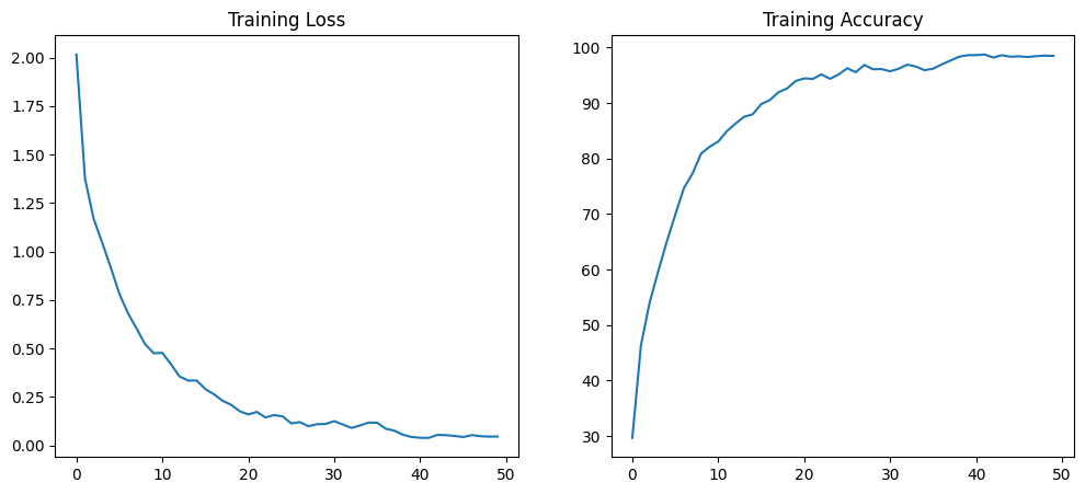
plt.bar(model.variances.keys(), model.variances.values())
plt.title("Variance per Layer")
plt.xticks(rotation=45)
plt.tight_layout()
plt.show()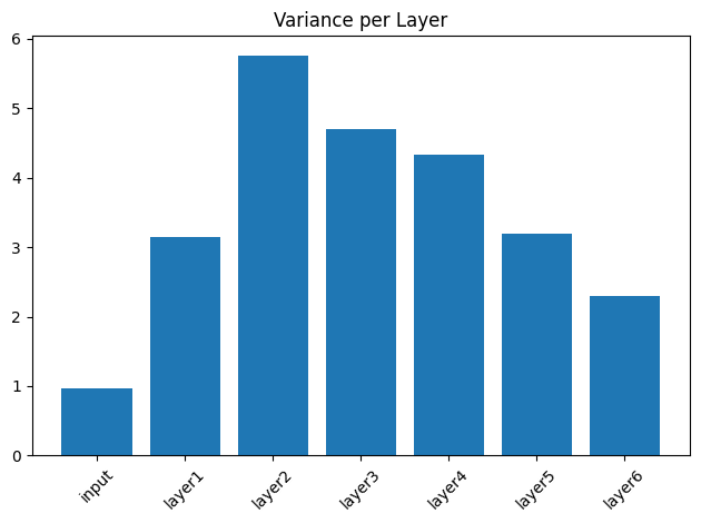
# This is a simple residual model with 5 residual branches in a row
class NNBatchNetwork(torch.nn.Module):
  def __init__(self, input_size, output_size, hidden_size=100):
    super(NNBatchNetwork, self).__init__()
    self.linear1 = nn.Linear(input_size, hidden_size)
    self.linear2 = nn.Linear(hidden_size, hidden_size)
    self.linear3 = nn.Linear(hidden_size, hidden_size)
    self.linear4 = nn.Linear(hidden_size, hidden_size)
    self.linear5 = nn.Linear(hidden_size, hidden_size)
    self.linear6 = nn.Linear(hidden_size, hidden_size)
    self.linear7 = nn.Linear(hidden_size, output_size)
    self.batch_norm1 = nn.BatchNorm1d(hidden_size)
    self.variances = {}

  def count_params(self):
    return sum([p.view(-1).shape[0] for p in self.parameters()])

  def forward(self, x):
    self.variances['input'] = get_variance("Input", x)
    f = self.linear1(x)
    self.variances['layer1'] = get_variance("First preactivation", f)
    f = self.batch_norm1(f)
    res1 = self.linear2(f.relu())
    self.variances['layer2'] = get_variance("After first layer", res1)
    res1 = self.batch_norm1(res1)
    res2 = self.linear3(res1.relu())
    self.variances['layer3'] = get_variance("After second layer", res2)
    res2 = self.batch_norm1(res2)
    res3 = self.linear4(res2.relu())
    self.variances['layer4'] = get_variance("After third layer", res3)
    res3 = self.batch_norm1(res3)
    res4 = self.linear5(res3.relu())
    self.variances['layer5'] = get_variance("After fourth layer", res4)
    res4 = self.batch_norm1(res4)
    res5 = self.linear6(res4.relu())
    self.variances['layer6'] = get_variance("After fifth layer", res5)
    res5 = self.batch_norm1(res5)
    self.variances['layer7'] = get_variance("After batch norm on fifth layer", res5)
return self.linear7(res5)# Define the model and run for one step
# Monitoring the variance at each point in the network
n_hidden = 100
n_input = 40
n_output = 10
model = NNBatchNetwork(n_input, n_output, n_hidden)
train_model(model, x_train, y_train, n_epochs=1)([2.0125549912452696], [28.849999999999998])# run the training loop for 50 epochs and monitor the variance at each point in the network
losses, accuracies = train_model(model, x_train, y_train, n_epochs=50)
print("The lowest loss is %f and the highest accuracy is %f" %
(min(losses), max(accuracies)))
plt.figure(figsize=(12, 5))
plt.subplot(1, 2, 1)
plt.plot(losses, label='Loss')
plt.title('Training Loss')
plt.subplot(1, 2, 2)
plt.plot(accuracies, label='Accuracy')
plt.title('Training Accuracy')
plt.show()The lowest loss is 0.033206 and the highest accuracy is 99.050000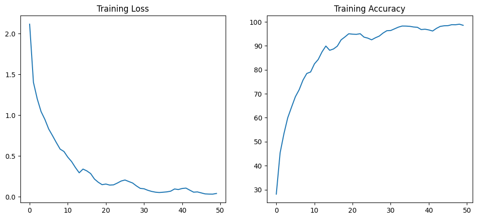
plt.bar(model.variances.keys(), model.variances.values())
plt.title("Variance per Layer")
plt.xticks(rotation=45)
plt.tight_layout()
plt.show()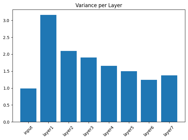
Comments