Gradient Descent
This is an explainer of one of the most important ideas in machine learning: Gradient Descent.
We will cover the following:
- What is Gradient Descent?
- Trial and Error
- Using Slope to Guide Us
- Math
- Code Example
- Visualizing the Loss Surface
- Summary
1. What is Gradient Descent?
Training a ML model refers to the proccess of minimize the mistakes the model makes. Gradient descent is the algorithm doing this task, it finds the values of a model’s parameters — its weights and biases — that leads for lower mistakes.
Think of it like standing on a hilly landscape and trying to reach the lowest point. Gradient descent gives you one simple rule: always take a step in the downhill direction. Keep doing that, step by step, and you will eventually reach the bottom.
In machine learning:
- The landscape is the loss surface — a mathematical surface representing how wrong the model is for every possible combination of weight values.
- The lowest point is the set of weights where the model makes the least error.
- Each step is a small update to the model’s weights.
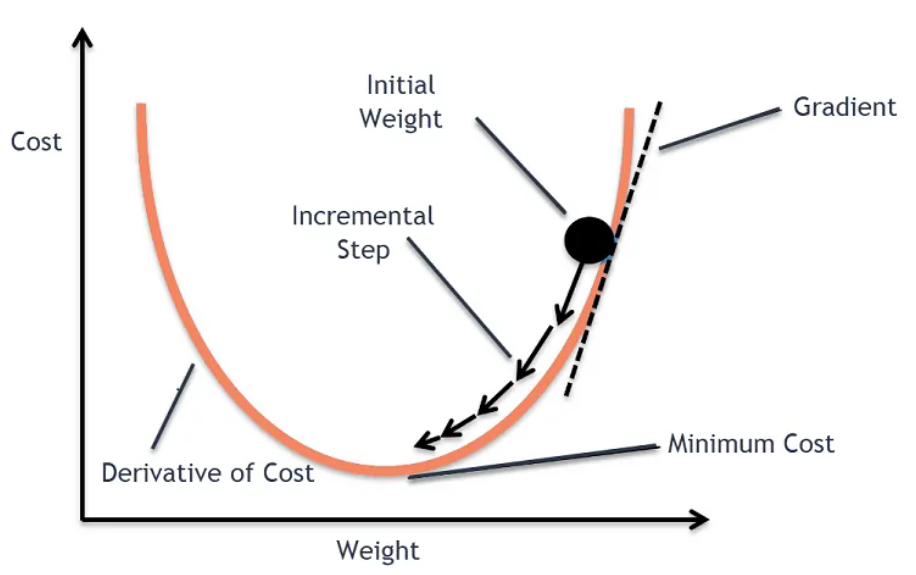
Image source: Abhay Singh on Medium
Understanding Gradient descent is the foundation for understanding how any model learns.
The loss function
Before we can reduce our mistakes, we need a way to measure them. This is the job of the loss function (also called the cost function or error function).
For a detailed explanation of loss functions refer to this: Loss Functions explainer.
To put it simply, the loss function takes the model’s predictions and compares them to the true answers, producing a single number: the loss. The higher the loss, the worse the model is performing.
A common loss function for regression tasks is Mean Squared Error (MSE):
\[L = \frac{1}{n} \sum_{i=1}^{n} (\hat{y}_i - y_i)^2\]
Where:
- \(n\) is the number of training examples
- \(\hat{y}_i\) is the model’s prediction for example \(i\)
- \(y_i\) is the true value for example \(i\)
Why using the square?
For two reasons:
- Makes all errors positive so they do not cancel each other out.
- It penalizes large errors more heavily than small ones.
Remember This! For every possible set of weight values, there is a corresponding loss value, this creats a loss surface. Gradient descent is the algorithm that searchs the surface to find the weights that make the loss as small as possible.
2. Trial and Error
Trying Random Changes
The is one lazy approach for finding the best weights combination that gives the lowest loss value, which is gussing.
We can try this: pick a random weight, compute the loss, pick another random weight, compute the loss again, and so on until we hit the lowest loss. But this is not efficient at all, it would take forever to find the best weights, especially as the number of weights increases. Also the loss surface is enormous and complex, it has many hills and valleys, so we need a smarter way to navigate it.
Why Random Updates Fail
One major problem of random updates is that they have no direction. They might take us uphill instead of downhill, which would increase the loss instead of decreasing it. We need a way to know which direction to go in order to reduce the loss.
How do we find the right direction?
This is where the concept of slope comes in.
3. Using Slope to Guide Us
Which Direction Reduces Error?
The slope of the loss surface at a given point tells us which way is uphill and which way is downhill. If we can calculate the slope, we can use it to guide our steps in the right direction.
Understanding Slope Intuitively
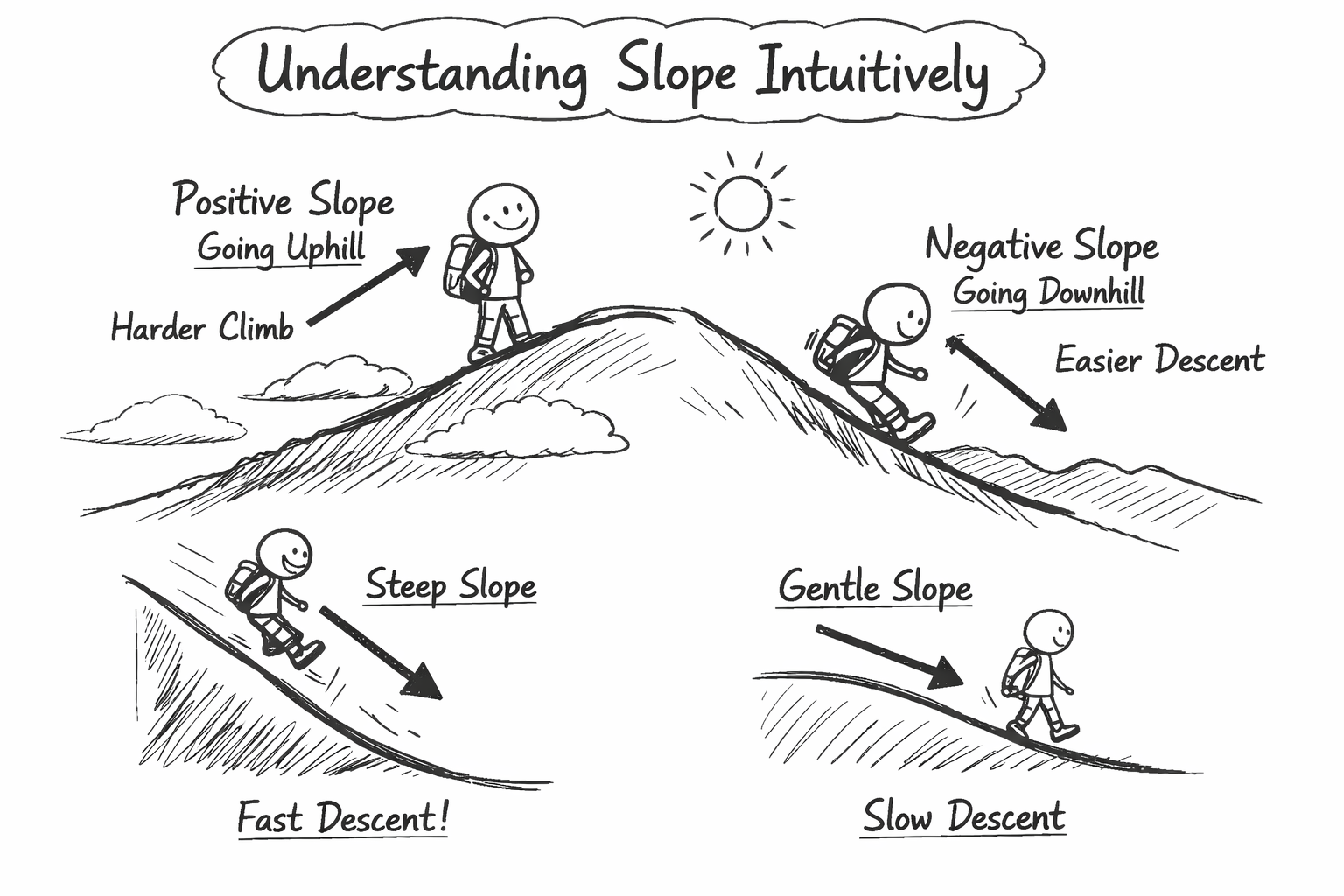
Imagine you are standing on a hill. The slope tells you how steep the hill is and which way is down. If the slope is positive, it means you are going uphill, and if it’s negative, it means you are going downhill. The steeper the slope, the faster you will go down if you take a step in that direction.
4. Math
Now that we have the intuition, let’s see how we can convert the above concepts into a mathematical form.
We mentioned that gradient descent is about taking steps in the direction of the steepest descent by moving in the loss surface. The slope is telling us which way is downhill, but how do we calculate it?
Giving the loss function: \[ L = \frac{1}{n} \sum_{i=1}^{n} (\hat{y}_i - y_i)^2 \]
For a simple linear model, the prediction \(\hat{y}_i\) is given by: \[ \hat{y}_i = w \cdot x_i \]
Where \(w\) is the weight and \(x_i\) is the input feature for example \(i\). Substituting this into the loss function gives us:
\[ L(w) = \frac{1}{n} \sum_{i=1}^{n} (w \cdot x_i - y_i)^2 \]
The slope of the loss function with respect to the weights is given by the gradient:
\[ \frac{\partial L}{\partial w} = \frac{2}{n} \sum_{i=1}^{n} (w \cdot x_i - y_i) \cdot x_i \]
The above formula is the slope of the loss surface at the current weight value \(w\). This is the key to finding the direction to move in order to reduce the loss.
The Update Step
Now that we have the gradient, we can use it to update our weights. The update rule for gradient descent is: \[ w_{\text{new}} = w_{\text{old}} - \alpha \cdot \frac{\partial L}{\partial w} \]
Where:
- \(w_{\text{new}}\) is the updated weight
- \(w_{\text{old}}\) is the current weight
- \(\alpha\) is the learning rate (How big our steps are).
Choosing the Learning Rate
The learning rate \(\alpha\) is a crucial hyperparameter in gradient descent. It determines how big our steps are. If \(\alpha\) is too small, the algorithm will take tiny steps, thus longer time to reach the minimum. If \(\alpha\) is too large, the algorithm might overshoot the minimum and never reach the minimum point.
5. Code Example
To apply the above concepts in code, we need to start with a simple dataset and a linear model.
We define a simple dataset with one input feature and one output: \[ x = [1, 2, 3, 4, 5] \] \[ y = 25 \]
Our goal is to find the weights \(w\) that best solve the equation: \[ w_1 \cdot x_1 + w_2 \cdot x_2 + w_3 \cdot x_3 + w_4 \cdot x_4 + w_5 \cdot x_5 = y \]
Thus:
\[ w_1 \cdot 1 + w_2 \cdot 2 + w_3 \cdot 3 + w_4 \cdot 4 + w_5 \cdot 5 = 25 \]
What are the values of \(w_1, w_2, w_3, w_4, w_5\) that satisfy the above equation?
The loss function for this problem is: \[ L(w) = \frac{1}{n} \sum_{i=1}^{n} (w_i \cdot x_i - y)^2 \]
We can plug in random values for weights: \[ w = [4.2, 3.6, 1.5, 0.7, 0.1] \]
\[ L(w) = \frac{1}{5} ((4.2 \cdot 1 - 25)^2 + (3.6 \cdot 2 - 25)^2 + (1.5 \cdot 3 - 25)^2 + (0.7 \cdot 4 - 25)^2 + (0.1 \cdot 5 - 25)^2) = 256.8 \]
The value \(256.8\) refers to the loss, we can see that is very high, we need to chose different weights to reduce the loss. But doing this by hand is not efficient, we need to use the gradient descent algorithm to find the best weights that minimize the loss.
In gradient descent, we take the gradient of the loss with respect to each weight, then keep updating the weights using the update rule until we reach the minimum loss.
The gradient of the loss with respect to each weight is given by: \[ \frac{\partial L}{\partial w_1} = \frac{2}{n} (w_1 x_1 - y) x_1 \]
And the same for \(w_2, w_3, w_4, w_5\).
Then we update the weights using the update rule: \[ w_{\text{new}} = w_{\text{old}} - \alpha \cdot \frac{\partial L}{\partial w} \]
Notice how the loss decreasing over time as we update the weights. Also notice how the algorithm modified the initial weights \([4.2, 3.6, 1.5, 0.7, 0.1]\) to find the best weights \([24.6, 12.4, 8.3, 6.25, 5.0]\) that minimize the loss to \(0.000000000000001\).
6. Visualizing the Loss Surface
If we fix weights \(w_2, w_3, w_4, w_5\) and vary only \(w_1\), we can visualize the loss surface as a function of \(w_1\). The gradient descent algorithm is trying to reach the lowest point on this curve by updating \(w_1\).
Summary
In summary, gradient descent is an optimization algorithm that helps us find the best weights for our model by moving through the loss surface and toward the minimum. It allows us to minimize the loss and improve our model’s performance by taking small steps in the right direction.
Comments