Linear Regression
The First Step Toward Machine Learning
This is an explainer of a fundamental part of Machine Learning and AI: Linear Regression.
We will discuss the following:
Definition
Linear regression is a statistical approach to predict a variable Y based on another variable X. It models the relationship between the two variables by fitting a straight line (the regression line) to the observed data. This line represents the best estimate of Y for any given value of X.
See the below image for example — this is a simple Linear relationship between temperature and Energy.
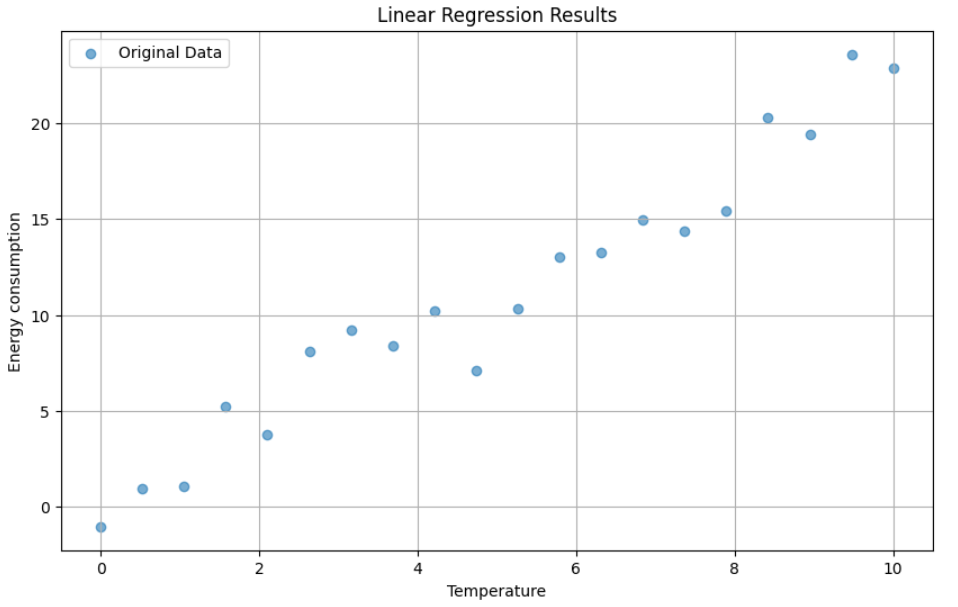
When the temperature (x-axis) increases, the value of energy consumption (y-axis) increases. This relationship can be modeled using a straight line. This line is telling us how the two variables are related: as one goes up, so does the other, in a predictable way. The line also can predict the value of energy consumption for a given temperature value. This is the simplest form of regression analysis.
Machine Learning involves finding the best-fitting line that describes the relationship between temperature and energy consumption, as shown in the example above. This process allows us to make predictions based on observed data. The question is: How to find the best-fitting line?
The Equation
Going back to the previous example, we consider the following:
- x : Tempreture
- y : Energy Consumption
The linear equation that represents the relationship between the two variables is:
\(y = w.x + b\)
We already know what \(x\) and \(y\) represents. But what is \(w\) and \(b\) ??
To get the intuition of these two variables, we will vary the value of \(w\) while keeping \(b\) constant, then observe how the line changes:
The line is changing when different values of \(w\) are plugged in. This should give you an intuition of the purpose of \(w\): it controls the slope of the line. A higher \(w\) means the line rises more steeply as \(x\) increases, while a lower (or negative) \(w\) means the line is flatter or slopes downward.
Similarly, \(b\) is called the intercept. It determines where the line crosses the \(y\)-axis. Changing \(b\) shifts the line up or down without changing its slope.
In summary:
- \(w\) (weight): Controls the angle or steepness of the line (the relationship strength between \(x\) and \(y\)).
- \(b\) (bias): Moves the line up or down.
Use Case
Now that we understand the line equation and its parameters, let’s see how to find the best values for \(w\) and \(b\) that fit our data. The goal is to choose \(w\) and \(b\) so that the line is as close as possible to all the data points.
In order to find those values, we need to start with the historical data collected on the input x (temperature) and the actual measured y value (energy consumption). Here is a preview of the historical data (training data):
| x (Tempreture) | Y (Energy Consumption) |
|---|---|
| 0.0 | 2.32 |
| 0.53 | 0.72 |
| 1.05 | 1.32 |
| 1.58 | 2.72 |
| 2.11 | 3.65 |
| 2.63 | 7.83 |
| 3.16 | 6.6 |
| 3.68 | 5.08 |
| 4.21 | 7.17 |
| 4.74 | 8.48 |
The approach in finding the values of w and b is to start with a random guess, then on each iteration change the values slowly until reaching the best results that fits the data.
How can we know that we reached the best results?
We need a tool—a mathematical function—that checks at the end of each iteration whether we have reached the best fit or not. This is called a loss function. The loss function measures how far we are from the true value; the returned value of this function is called error. The bigger the value, the farther we are from the best fit.
A common loss function for linear regression is the Mean Squared Error (MSE), which is calculated as:
\[ \text{MSE} = \frac{1}{n} \sum_{i=1}^{n} (y_i - \hat{y}_i)^2 \]
Where:
\(y_i\) is the actual value,
\(\hat{y}_i\) is the predicted value from our line,
\(n\) is the number of data points.
What does the iqueation represents? - For each iteration, predict the value of \(\hat{y}_i\) then subtract it from the true value \(y_i\) (calculate the error), then after all iterations average all errors collected by dividing by the total number of points \(n\).
Training a Linear Regression Model
In this section I will guide you on how to train a simple linear regression model..
Remeber that training in machine learning requires the following:
- Training Data: A set of input-output pairs (in our case, temperature and energy consumption).
- A Model: The linear equation \(y = wx + b\).
- A Loss Function: To measure how well the model predicts the data (we use Mean Squared Error).
- An Optimization Algorithm: To adjust \(w\) and \(b\) to minimize the loss (commonly, Gradient Descent).
Let’s see how this works in practice using Python:
Don’t panic on the numbers, we are only defining numbers that will be used for training. We are only training on 20 sample points, but in actual scenarios millions of records used for training, the more training data the better the results we get.
If you’re not quite ready for the example above, I’ve created a simpler explainer to help you build intuition about what actually happens during training and what “training” really means.
👉 See the Simple Training Intuition page
After defining the training data above, here is a sample for preview:
Remember this is our model:
\[ y = w.X + b \]
For a start we need an initial values of \(w\) and \(b\), lets set them to:
These are totally random values, you can pick different values if you want.
Now with the above values of \(w\) and \(b\), lets see the how the line fits the \(X\) and \(y\) points defined earlier :
You can adjust the values of w and b and then rerun the above cell to see how the line changes.
Math
REMEMBER, training is finding the best values of \(w\) and \(b\) that will fit the data. For that we will use the gradient decent technique to update the weights on each iteration.
What is gradient decent?
It is a mathematical approach that helps the model learn by slowly adjusting \(w\) and \(b\) so the loss gets smaller and smaller. At each step, gradient descent checks how far off the prediction is, then change the weights in the direction that makes the error less. By repeating this process, the model gets closer to the best fit.
For that we need to do the following steps on each iteration:
Start with a random guess for \(w\) and \(b\).
Get \(\hat{y}_i\) (the predicted value) by plugging to the model equation (\(y = wx + b\)).
Get the Loss (How far the predicted value from the target?).
Using the gradient of \(w\) and \(b\), update their values.
Repeat the process.
Only one thing remains before turning everything to code, What is the gradient?
The gradient is telling us how much the loss will change if we tweak \(w\) or \(b\) just a little. It points in the direction where the loss gets smaller, and this is the purpose of the whole process; we need to find the best values of weights that leads to smaller loss.
In math terms,,
To find the gradient of \(w\) for example, we start with the loss function:
\[ \text{MSE} = \frac{1}{n} \sum_{i=1}^{n} (y_i - \hat{y}_i)^2 \]
Substite \(\hat{y}_i\) with the model equation \(\hat{y}_i = w.x + b\)
\[ \text{MSE} = \text{Loss}= \frac{1}{n} \sum_{i=1}^{n} (y_i - w.x+b)^2 \]
Compute the gradient with respect to \(w\) (How much the loss is changing when \(w\) changes?)
\[ \frac{\partial \text{Loss}}{\partial w} = 2(y_{\text{i}} - w x + b) \cdot x \]
The summation symbol \(\sum_{i=1}^{n}\) is used when calculating the loss over all data points. Here, we’re working with just one example, so the sum disappears from the equation.
The same process for the gradient of \(b\) :
\[ \frac{\partial \text{Loss}}{\partial b} = 2(y_{\text{i}} - w x + b) \]
Now we use these gradient values to get the updated values of the weights:
\[ w_{new} = w_{old} - lr \cdot \frac{\partial \text{Loss}}{\partial w} \]
\[ b_{new} = b_{old} - lr \cdot \frac{\partial \text{Loss}}{\partial b} \]
The \(lr\) in the equation stands for learning rate. It controls how big a step we take when updating \(w\). A small learning rate means slower, careful steps; a large learning rate means faster, bigger steps. Choosing the right learning rate helps the model learn efficiently.
Code
Now that we have the mathematical tools and intuition of how training works, lets turn everything into code, and see how the training process will modify the initial values of w and b until it finds the best fit for the line:
Start with defining inital values:
Define the Loss function and the gradient function:
If you checked the other simple explainer, we used only a single x and y values. Here we have a list of X values and Y values.
👉 See the Simple Training Intuition page
Because we have a list of X and Y values, in each epoch we use all values of X to predict a list of Y predictions. Then, we calculate the average gradient across all points and use it to update the weights. This way, the model learns from the whole dataset at once, not just a single example.
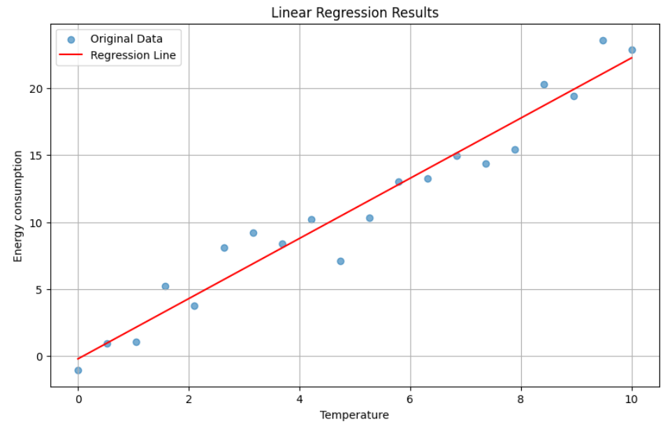
Using the final weights we found, plot the line and see how it fits the data:
Notice In the below graph the difference between our initail guess we made in the beggining of this explainer, and the position of the line the model predicted after training.
Summary
In this explainer, we learned how linear regression works by fitting a straight line to data using the equation \(y=w.x + b\). The start was with a random guess of the values w and b (weights), then using the gradient decent approach, we looped over the data updating the values of weights for a certin number of epochs. The results show the best fitting line.
Comments