The gradient of \(w_1\) is: \[ \frac{\partial L}{\partial w_1} = (w_1 x_1 + w_2 x_2 + w_3 x_3 + w_4 x_4 + w_5 x_5 + b - y) \cdot x_1 \]
The gradient of \(b\) is: \[ \frac{\partial L}{\partial b} = (w_1 x_1 + w_2 x_2 + w_3 x_3 + w_4 x_4 + w_5 x_5 + b - y) \]
Show Code
import numpy as np# Datasetx = np.array([1, 2, 3, 4, 5])y =25# Initial weightsw = np.array([4.2, 3.6, 1.5, 0.7, 0.1])b =0.0# Learning ratealpha =0.01# Compute the lossdef compute_loss(w, b, x, y):return np.mean((w * x + b - y) **2) # the mean if we have multiple data points# Compute the gradient (This is for a single data point)def compute_gradient(w, b, x, y): error = np.dot(w, x) + b - y dw =2* error * x # gradient w.r.t each weight db =2* error # gradient w.r.t biasreturn dw, db# Update weightsdef update_weights(w, b, x, y, alpha): dw, db = compute_gradient(w, b, x, y) w = w - alpha * dw b = b - alpha * dbreturn w, b# Training loopfor epoch inrange(1000): loss = compute_loss(w, b, x, y) w, b = update_weights(w, b, x, y, alpha)if epoch %100==0:print(f"Epoch {epoch}: Loss = {loss}")print(f"Final weights: {w}")print(f"Final bias: {b}")print(f"Final loss: {compute_loss(w, b, x, y)}")#multiply weights with x:print(f"Prediction: {np.dot(w, x) + b}")
Epoch 0: Loss = 452.56399999999996
Epoch 100: Loss = 398.9825051020408
Epoch 200: Loss = 398.9825051020408
Epoch 300: Loss = 398.9825051020408
Epoch 400: Loss = 398.9825051020408
Epoch 500: Loss = 398.9825051020408
Epoch 600: Loss = 398.9825051020408
Epoch 700: Loss = 398.9825051020408
Epoch 800: Loss = 398.9825051020408
Epoch 900: Loss = 398.9825051020408
Final weights: [4.30357143 3.80714286 1.81071429 1.11428571 0.61785714]
Final bias: 0.10357142857142854
Final loss: 398.9825051020408
Prediction: 25.0
Before moving forward, lets create data with multiple examples.
#Dataset with multiple examplesx = np.array([[1, 2, 3, 4, 5], [2, 3, 4, 5, 6], [3, 4, 5, 6, 7]])y = np.array([25, 30, 35])w = np.zeros(x.shape[1]) # Initialize weights to zerob =0.0alpha =0.01# Compute the lossdef compute_loss(w, b, x, y):return np.mean((np.dot(x, w) + b - y) **2)def compute_gradient(w, b, x, y): errors = np.dot(x, w) + b - y # shape (3,) — one error per example dw = (2/len(x)) * np.dot(x.T, errors) # shape (5,) db = (2/len(x)) * np.sum(errors) # scalarreturn dw, dbdef update_weights(w, b, x, y, alpha): dw, db = compute_gradient(w, b, x, y) w = w - alpha * dw b = b - alpha * dbreturn w, bfor epoch inrange(1000): loss = compute_loss(w, b, x, y) w, b = update_weights(w, b, x, y, alpha)if epoch %100==0:print(f"Epoch {epoch}: Loss = {loss}")print(f"Final weights: {w}")print(f"Final bias: {b}")print(f"Predictions: {np.dot(x, w) + b}")print(f"Targets: {y}")
Epoch 0: Loss = 916.6666666666666
Epoch 100: Loss = 0.3542681599414232
Epoch 200: Loss = 0.07389895348457104
Epoch 300: Loss = 0.015415033100318507
Epoch 400: Loss = 0.0032155157046107573
Epoch 500: Loss = 0.0006707440184727005
Epoch 600: Loss = 0.00013991458280599502
Epoch 700: Loss = 2.918563556681734e-05
Epoch 800: Loss = 6.088009600987926e-06
Epoch 900: Loss = 1.269935027346966e-06
Final weights: [-0.81758997  0.09126705  1.00012407  1.9089811   2.81783812]
Final bias: 0.9088570222521724
Predictions: [24.99928835 29.99990871 35.00052908]
Targets:     [25 30 35]
Why x.T?
We need the first feature (\(x_1\)) of all examples to be in the first row, becasue the gradient is computed as the dot product of the error and the input features. If we have the features in columns, we can easily compute the gradient for all examples at once using matrix multiplication.
Training real data
Let’s test the above implementation on the real data. Can the above implementation get accurate results for a real dataset?
Show Code
# import datasetfrom sklearn.datasets import load_diabetesdata = load_diabetes()X, y = data.data, data.target#split dataset into train and testfrom sklearn.model_selection import train_test_splitX_train, X_test, y_train, y_test = train_test_split(X, y, test_size=0.2, random_state=42)
Show Code
#print the first 5 examples in a dataframeimport pandas as pddf = pd.DataFrame(X_train, columns=data.feature_names)df.head()
age
sex
bmi
bp
s1
s2
s3
s4
s5
s6
0
0.070769
0.050680
0.012117
0.056301
0.034206
0.049416
-0.039719
0.034309
0.027364
-0.001078
1
-0.009147
0.050680
-0.018062
-0.033213
-0.020832
0.012152
-0.072854
0.071210
0.000272
0.019633
2
0.005383
-0.044642
0.049840
0.097615
-0.015328
-0.016345
-0.006584
-0.002592
0.017036
-0.013504
3
-0.027310
-0.044642
-0.035307
-0.029770
-0.056607
-0.058620
0.030232
-0.039493
-0.049872
-0.129483
4
-0.023677
-0.044642
-0.065486
-0.081413
-0.038720
-0.053610
0.059685
-0.076395
-0.037129
-0.042499
Features in the diabetes dataset:
Column
Full Name
Description
age
Age
Age of the patient
sex
Sex
Sex of the patient
bmi
Body Mass Index
Weight relative to height
bp
Blood Pressure
Average blood pressure
s1
TC
Total cholesterol
s2
LDL
Low-density lipoprotein
s3
HDL
High-density lipoprotein
s4
TCH
Total cholesterol / HDL ratio
s5
LTG
Log of serum triglycerides
s6
GLU
Blood sugar level
The values like 0.038076, -0.034821 are because sklearn already normalized them — each feature has been scaled to have:
Mean = 0
Standard deviation = 1
Show Code
print(y[:5])
[151. 75. 141. 206. 135.]
Show Code
b =0.0# Compute the lossdef compute_loss(w, b, x, y):return np.mean((np.dot(x, w) + b - y) **2)def compute_gradient(w, b, x, y): errors = np.dot(x, w) + b - y # shape (3,) — one error per example dw = (2/len(x)) * np.dot(x.T, errors) # shape (10,) db = (2/len(x)) * np.sum(errors) # scalarreturn dw, dbdef update_weights(w, b, x, y, alpha): dw, db = compute_gradient(w, b, x, y) w = w - alpha * dw b = b - alpha * dbreturn w, b
Show Code
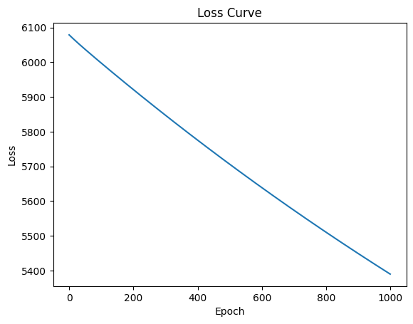
#store losses for plottinglosses = []alpha =0.01w = np.zeros(X_train.shape[1]) # Initialize weights to zero# training loopfor epoch inrange(1000): loss = compute_loss(w, b, X_train, y_train) w, b = update_weights(w, b, X_train, y_train, alpha) losses.append(loss)if epoch %100==0:print(f"Epoch {epoch}: Loss = {loss}")#plot the loss curveimport matplotlib.pyplot as pltplt.plot(losses)plt.xlabel('Epoch')plt.ylabel('Loss')plt.title('Loss Curve')plt.show()
Epoch 0: Loss = 6078.967813535314
Epoch 100: Loss = 5997.582985597988
Epoch 200: Loss = 5921.177398303041
Epoch 300: Loss = 5847.190151819955
Epoch 400: Loss = 5775.497046711073
Epoch 500: Loss = 5706.019503961029
Epoch 600: Loss = 5638.682415619815
Epoch 700: Loss = 5573.413309446693
Epoch 800: Loss = 5510.1422434676015
Epoch 900: Loss = 5448.801716577623
We notice from the abvove that the model is not performing well. The loss is not decreasing and the predictions are not close to the actual values.
We need to improve the training process by: - Randomly initializing the weights and bias
Reducing the learning rate
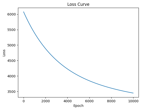
Show Code
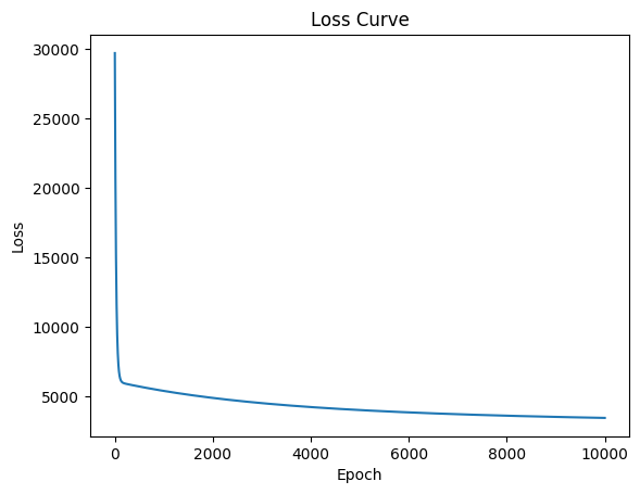
#store losses for plottinglosses = []alpha =0.01w = np.random.randn(X_train.shape[1]) *0.01# small random values# training loopfor epoch inrange(10000): loss = compute_loss(w, b, X_train, y_train) w, b = update_weights(w, b, X_train, y_train, alpha) losses.append(loss)if epoch %100==0:print(f"Epoch {epoch}: Loss = {loss}")#plot the loss curveimport matplotlib.pyplot as pltplt.plot(losses)plt.xlabel('Epoch')plt.ylabel('Loss')plt.title('Loss Curve')plt.show()
Epoch 0: Loss = 6076.474836574767
Epoch 100: Loss = 5997.59499482191
Epoch 200: Loss = 5921.2326574172075
Epoch 300: Loss = 5847.245383693941
Epoch 400: Loss = 5775.551507061216
Epoch 500: Loss = 5706.073196041579
Epoch 600: Loss = 5638.735355362369
Epoch 700: Loss = 5573.465512551738
Epoch 800: Loss = 5510.193725192475
Epoch 900: Loss = 5448.852491747228
Epoch 1000: Loss = 5389.376665541143
Epoch 1100: Loss = 5331.7033717851
Epoch 1200: Loss = 5275.771927531907
Epoch 1300: Loss = 5221.523764461674
Epoch 1400: Loss = 5168.902354396241
Epoch 1500: Loss = 5117.853137446141
Epoch 1600: Loss = 5068.323452696923
Epoch 1700: Loss = 5020.262471345028
Epoch 1800: Loss = 4973.621132196499
Epoch 1900: Loss = 4928.352079445013
Epoch 2000: Loss = 4884.4096026484995
Epoch 2100: Loss = 4841.749578826645
Epoch 2200: Loss = 4800.329416604203
Epoch 2300: Loss = 4760.108002327755
Epoch 2400: Loss = 4721.045648086098
Epoch 2500: Loss = 4683.1040415669295
Epoch 2600: Loss = 4646.246197684861
Epoch 2700: Loss = 4610.436411918091
Epoch 2800: Loss = 4575.640215293314
Epoch 2900: Loss = 4541.824330960554
Epoch 3000: Loss = 4508.956632301666
Epoch 3100: Loss = 4477.006102518284
Epoch 3200: Loss = 4445.942795646865
Epoch 3300: Loss = 4415.7377989503575
Epoch 3400: Loss = 4386.363196637797
Epoch 3500: Loss = 4357.792034864874
Epoch 3600: Loss = 4329.998287970148
Epoch 3700: Loss = 4302.956825903229
Epoch 3800: Loss = 4276.643382802739
Epoch 3900: Loss = 4251.034526683425
Epoch 4000: Loss = 4226.10763019316
Epoch 4100: Loss = 4201.840842402028
Epoch 4200: Loss = 4178.213061586983
Epoch 4300: Loss = 4155.2039089768505
Epoch 4400: Loss = 4132.793703423759
Epoch 4500: Loss = 4110.963436968196
Epoch 4600: Loss = 4089.6947512661195
Epoch 4700: Loss = 4068.96991484763
Epoch 4800: Loss = 4048.7718011777933
Epoch 4900: Loss = 4029.0838674912743
Epoch 5000: Loss = 4009.890134373396
Epoch 5100: Loss = 3991.175166061249
Epoch 5200: Loss = 3972.9240514393928
Epoch 5300: Loss = 3955.122385705588
Epoch 5400: Loss = 3937.756252682872
Epoch 5500: Loss = 3920.812207755135
Epoch 5600: Loss = 3904.2772614041537
Epoch 5700: Loss = 3888.1388633268048
Epoch 5800: Loss = 3872.3848871119835
Epoch 5900: Loss = 3857.0036154574154
Epoch 6000: Loss = 3841.983725907285
Epoch 6100: Loss = 3827.3142770922846
Epoch 6200: Loss = 3812.9846954543054
Epoch 6300: Loss = 3798.984762438673
Epoch 6400: Loss = 3785.3046021373743
Epoch 6500: Loss = 3771.9346693673483
Epoch 6600: Loss = 3758.8657381684848
Epoch 6700: Loss = 3746.0888907064686
Epoch 6800: Loss = 3733.595506566194
Epoch 6900: Loss = 3721.3772524219276
Epoch 7000: Loss = 3709.4260720709226
Epoch 7100: Loss = 3697.734176817641
Epoch 7200: Loss = 3686.294036196189
Epoch 7300: Loss = 3675.0983690190333
Epoch 7400: Loss = 3664.140134740463
Epoch 7500: Loss = 3653.412525123671
Epoch 7600: Loss = 3642.908956200761
Epoch 7700: Loss = 3632.623060515295
Epoch 7800: Loss = 3622.5486796374344
Epoch 7900: Loss = 3612.6798569420366
Epoch 8000: Loss = 3603.0108306404154
Epoch 8100: Loss = 3593.536027056818
Epoch 8200: Loss = 3584.250054140981
Epoch 8300: Loss = 3575.147695208411
Epoch 8400: Loss = 3566.2239029003786
Epoch 8500: Loss = 3557.473793355847
Epoch 8600: Loss = 3548.8926405878565
Epoch 8700: Loss = 3540.475871057171
Epoch 8800: Loss = 3532.219058436192
Epoch 8900: Loss = 3524.117918556445
Epoch 9000: Loss = 3516.1683045331647
Epoch 9100: Loss = 3508.366202060707
Epoch 9200: Loss = 3500.707724872788
Epoch 9300: Loss = 3493.189110361716
Epoch 9400: Loss = 3485.8067153510106
Epoch 9500: Loss = 3478.5570120160155
Epoch 9600: Loss = 3471.4365839472507
Epoch 9700: Loss = 3464.4421223515074
Epoch 9800: Loss = 3457.5704223858047
Epoch 9900: Loss = 3450.8183796195267
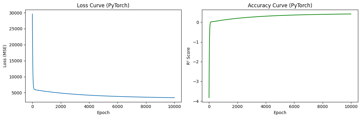
Let’s test the above implementation on pytorch. Can we get the same results using pytorch?
Show Code
import torchimport torch.nn as nn# Convert to tensorsX_tensor = torch.tensor(X_train, dtype=torch.float32)y_tensor = torch.tensor(y_train, dtype=torch.float32).view(-1, 1) # shape (442, 1)# Define model — same as ours: linear layer (weights + bias)model = nn.Linear(X_train.shape[1], 1) # 10 inputs, 1 output# Loss function — same as ours: MSEloss_fn = nn.MSELoss()# Optimizer — same as ours: gradient descentoptimizer = torch.optim.SGD(model.parameters(), lr=0.01)# Training loop# PyTorch Implementation - Accuracy Curve (R²)losses = []r2_scores = []for epoch inrange(10000): y_pred = model(X_tensor) loss = loss_fn(y_pred, y_tensor) optimizer.zero_grad() loss.backward() optimizer.step()# compute R² every epochwith torch.no_grad(): X_test_tensor = torch.tensor(X_test, dtype=torch.float32) y_test_tensor = torch.tensor(y_test, dtype=torch.float32).view(-1, 1) preds = model(X_test_tensor).squeeze().numpy() r2 = r2_score(y_test, preds) losses.append(loss.item()) r2_scores.append(r2)# Plot both curves side by sidefig, (ax1, ax2) = plt.subplots(1, 2, figsize=(12, 4))ax1.plot(losses)ax1.set_xlabel('Epoch')ax1.set_ylabel('Loss (MSE)')ax1.set_title('Loss Curve (PyTorch)')ax2.plot(r2_scores, color='green')ax2.set_xlabel('Epoch')ax2.set_ylabel('R² Score')ax2.set_title('Accuracy Curve (PyTorch)')plt.tight_layout()plt.show()print(f"Final R²: {r2_scores[-1]:.4f}")print(f"Final RMSE: {np.sqrt(losses[-1]):.2f}")
Final R²:   0.4167
Final RMSE: 58.69
Improt model class defined in model_functions.py
Show Code
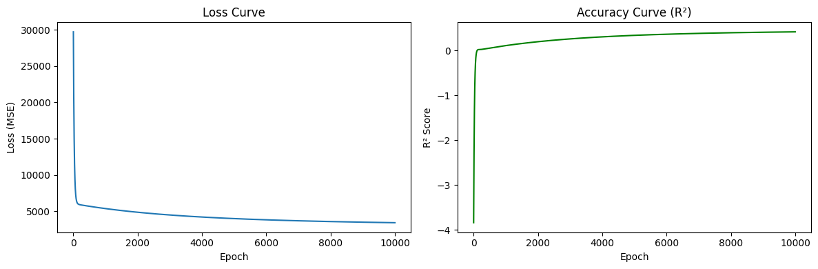
from model_functions import MyModelmodel = MyModel(alpha=0.01, epochs=10000)model.fit(X_train, y_train)model.plot_loss()
Epoch 0: Loss = 29711.4162
Epoch 100: Loss = 6409.4053
Epoch 200: Loss = 5924.7243
Epoch 300: Loss = 5843.6582
Epoch 400: Loss = 5771.9388
Epoch 500: Loss = 5702.5559
Epoch 600: Loss = 5635.3125
Epoch 700: Loss = 5570.1342
Epoch 800: Loss = 5506.9511
Epoch 900: Loss = 5445.6957
Epoch 1000: Loss = 5386.3030
Epoch 1100: Loss = 5328.7102
Epoch 1200: Loss = 5272.8567
Epoch 1300: Loss = 5218.6841
Epoch 1400: Loss = 5166.1359
Epoch 1500: Loss = 5115.1576
Epoch 1600: Loss = 5065.6967
Epoch 1700: Loss = 5017.7023
Epoch 1800: Loss = 4971.1255
Epoch 1900: Loss = 4925.9191
Epoch 2000: Loss = 4882.0373
Epoch 2100: Loss = 4839.4360
Epoch 2200: Loss = 4798.0729
Epoch 2300: Loss = 4757.9068
Epoch 2400: Loss = 4718.8980
Epoch 2500: Loss = 4681.0084
Epoch 2600: Loss = 4644.2010
Epoch 2700: Loss = 4608.4402
Epoch 2800: Loss = 4573.6915
Epoch 2900: Loss = 4539.9216
Epoch 3000: Loss = 4507.0986
Epoch 3100: Loss = 4475.1915
Epoch 3200: Loss = 4444.1703
Epoch 3300: Loss = 4414.0061
Epoch 3400: Loss = 4384.6712
Epoch 3500: Loss = 4356.1386
Epoch 3600: Loss = 4328.3822
Epoch 3700: Loss = 4301.3771
Epoch 3800: Loss = 4275.0989
Epoch 3900: Loss = 4249.5243
Epoch 4000: Loss = 4224.6307
Epoch 4100: Loss = 4200.3963
Epoch 4200: Loss = 4176.8000
Epoch 4300: Loss = 4153.8214
Epoch 4400: Loss = 4131.4408
Epoch 4500: Loss = 4109.6394
Epoch 4600: Loss = 4088.3988
Epoch 4700: Loss = 4067.7013
Epoch 4800: Loss = 4047.5297
Epoch 4900: Loss = 4027.8676
Epoch 5000: Loss = 4008.6990
Epoch 5100: Loss = 3990.0084
Epoch 5200: Loss = 3971.7811
Epoch 5300: Loss = 3954.0025
Epoch 5400: Loss = 3936.6589
Epoch 5500: Loss = 3919.7368
Epoch 5600: Loss = 3903.2232
Epoch 5700: Loss = 3887.1055
Epoch 5800: Loss = 3871.3718
Epoch 5900: Loss = 3856.0102
Epoch 6000: Loss = 3841.0095
Epoch 6100: Loss = 3826.3588
Epoch 6200: Loss = 3812.0474
Epoch 6300: Loss = 3798.0652
Epoch 6400: Loss = 3784.4024
Epoch 6500: Loss = 3771.0493
Epoch 6600: Loss = 3757.9968
Epoch 6700: Loss = 3745.2360
Epoch 6800: Loss = 3732.7583
Epoch 6900: Loss = 3720.5553
Epoch 7000: Loss = 3708.6190
Epoch 7100: Loss = 3696.9416
Epoch 7200: Loss = 3685.5156
Epoch 7300: Loss = 3674.3338
Epoch 7400: Loss = 3663.3890
Epoch 7500: Loss = 3652.6746
Epoch 7600: Loss = 3642.1839
Epoch 7700: Loss = 3631.9106
Epoch 7800: Loss = 3621.8484
Epoch 7900: Loss = 3611.9916
Epoch 8000: Loss = 3602.3343
Epoch 8100: Loss = 3592.8709
Epoch 8200: Loss = 3583.5961
Epoch 8300: Loss = 3574.5047
Epoch 8400: Loss = 3565.5916
Epoch 8500: Loss = 3556.8519
Epoch 8600: Loss = 3548.2810
Epoch 8700: Loss = 3539.8742
Epoch 8800: Loss = 3531.6271
Epoch 8900: Loss = 3523.5355
Epoch 9000: Loss = 3515.5953
Epoch 9100: Loss = 3507.8023
Epoch 9200: Loss = 3500.1528
Epoch 9300: Loss = 3492.6429
Epoch 9400: Loss = 3485.2691
Epoch 9500: Loss = 3478.0278
Epoch 9600: Loss = 3470.9156
Epoch 9700: Loss = 3463.9292
Epoch 9800: Loss = 3457.0654
Epoch 9900: Loss = 3450.3211
Improve the model by adding an activation function
First sample: \[ x = [x_1, x_2, x_3, x_4, x_5, x_6, x_7, x_8, x_9, x_{10}] \]\[ x = [0.070769,0.050680,0.012117,0.056301,0.034206,0.049416,-0.039719,0.034309,0.027364,-0.001078] \]\[ y = 144.0\]
import importlibimport model_functionsimportlib.reload(model_functions)from model_functions import MyModelReLUmodel = MyModelReLU(alpha=0.01, epochs=10000)model.fit(X_train, y_train)model.plot_loss() y_pred = model.predict(X_test) # ⚠️ need to override predict too!
Epoch 0: Loss = 29711.2339
Epoch 100: Loss = 6420.0955
Epoch 200: Loss = 5925.5228
Epoch 300: Loss = 5844.2659
Epoch 400: Loss = 5772.5269
Epoch 500: Loss = 5703.1279
Epoch 600: Loss = 5635.8690
Epoch 700: Loss = 5570.6756
Epoch 800: Loss = 5507.4778
Epoch 900: Loss = 5446.2083
Epoch 1000: Loss = 5386.8020
Epoch 1100: Loss = 5329.1960
Epoch 1200: Loss = 5273.3297
Epoch 1300: Loss = 5219.1447
Epoch 1400: Loss = 5166.5845
Epoch 1500: Loss = 5115.5946
Epoch 1600: Loss = 5066.1224
Epoch 1700: Loss = 5018.1171
Epoch 1800: Loss = 4971.5298
Epoch 1900: Loss = 4926.3130
Epoch 2000: Loss = 4882.4213
Epoch 2100: Loss = 4839.8105
Epoch 2200: Loss = 4798.4380
Epoch 2300: Loss = 4758.2629
Epoch 2400: Loss = 4719.2454
Epoch 2500: Loss = 4681.3473
Epoch 2600: Loss = 4644.5316
Epoch 2700: Loss = 4608.7628
Epoch 2800: Loss = 4574.0063
Epoch 2900: Loss = 4540.2290
Epoch 3000: Loss = 4507.3987
Epoch 3100: Loss = 4475.4845
Epoch 3200: Loss = 4444.4565
Epoch 3300: Loss = 4414.2857
Epoch 3400: Loss = 4384.9443
Epoch 3500: Loss = 4356.4054
Epoch 3600: Loss = 4328.6430
Epoch 3700: Loss = 4301.6320
Epoch 3800: Loss = 4275.3481
Epoch 3900: Loss = 4249.7680
Epoch 4000: Loss = 4224.8690
Epoch 4100: Loss = 4200.6293
Epoch 4200: Loss = 4177.0279
Epoch 4300: Loss = 4154.0443
Epoch 4400: Loss = 4131.6590
Epoch 4500: Loss = 4109.8529
Epoch 4600: Loss = 4088.6078
Epoch 4700: Loss = 4067.9058
Epoch 4800: Loss = 4047.7300
Epoch 4900: Loss = 4028.0637
Epoch 5000: Loss = 4008.8910
Epoch 5100: Loss = 3990.1966
Epoch 5200: Loss = 3971.9654
Epoch 5300: Loss = 3954.1831
Epoch 5400: Loss = 3936.8359
Epoch 5500: Loss = 3919.9103
Epoch 5600: Loss = 3903.3932
Epoch 5700: Loss = 3887.2723
Epoch 5800: Loss = 3871.5353
Epoch 5900: Loss = 3856.1706
Epoch 6000: Loss = 3841.1668
Epoch 6100: Loss = 3826.5130
Epoch 6200: Loss = 3812.1988
Epoch 6300: Loss = 3798.2138
Epoch 6400: Loss = 3784.5481
Epoch 6500: Loss = 3771.1924
Epoch 6600: Loss = 3758.1373
Epoch 6700: Loss = 3745.3739
Epoch 6800: Loss = 3732.8937
Epoch 6900: Loss = 3720.6882
Epoch 7000: Loss = 3708.7496
Epoch 7100: Loss = 3697.0699
Epoch 7200: Loss = 3685.6416
Epoch 7300: Loss = 3674.4576
Epoch 7400: Loss = 3663.5107
Epoch 7500: Loss = 3652.7942
Epoch 7600: Loss = 3642.3015
Epoch 7700: Loss = 3632.0261
Epoch 7800: Loss = 3621.9621
Epoch 7900: Loss = 3612.1033
Epoch 8000: Loss = 3602.4442
Epoch 8100: Loss = 3592.9790
Epoch 8200: Loss = 3583.7024
Epoch 8300: Loss = 3574.6093
Epoch 8400: Loss = 3565.6945
Epoch 8500: Loss = 3556.9532
Epoch 8600: Loss = 3548.3806
Epoch 8700: Loss = 3539.9722
Epoch 8800: Loss = 3531.7237
Epoch 8900: Loss = 3523.6306
Epoch 9000: Loss = 3515.6888
Epoch 9100: Loss = 3507.8944
Epoch 9200: Loss = 3500.2435
Epoch 9300: Loss = 3492.7323
Epoch 9400: Loss = 3485.3571
Epoch 9500: Loss = 3478.1145
Epoch 9600: Loss = 3471.0010
Epoch 9700: Loss = 3464.0133
Epoch 9800: Loss = 3457.1483
Epoch 9900: Loss = 3450.4027
Improve the model by adding a second layer
Each hidden neuron is just like your single-layer case: a weighted sum plus (optionally) an activation function.
#forward passdef forward_pass(w, b, x):return np.dot(x, w) + b# Compute the lossdef compute_loss(w, b, x, y):return np.mean((forward_pass(w, b, x) - y) **2)def compute_gradient(w, b, x, y): errors = forward_pass(w, b, x) - y # shape (3,) — one error per example dw = (2/len(x)) * np.dot(x.T, errors) # shape (10,) db = (2/len(x)) * np.sum(errors) # scalarreturn dw, dbdef update_weights(w, b, x, y, alpha): dw, db = compute_gradient(w, b, x, y) w = w - alpha * dw b = b - alpha * dbreturn w, b
Show Code
# define a weight initialization function matrix of previous layer to current layerdef initialize_weights(hidden_size, input_size):return np.random.randn(input_size, hidden_size) *0.01# small random valuesinitialize_weights(3, 3)
X = np.array([[1, 2, 3], [4, 5, 6], [7, 8, 9]])Y = np.array([10, 28, 40])x_one_example = np.array([1, 2, 3])w = initialize_weights(3, 3)b = np.zeros(3) # one bias per hidden neuronprint("For one example:", forward_pass(w, b, x_one_example), "... These are the activations of the hidden layer.")print("==="*20)print("For multiple examples:\n", forward_pass(w, b, X))
For one example: [ 0.01380295 -0.0005757  -0.01468555] ... These are the activations of the hidden layer.
============================================================
For multiple examples:
 [[ 0.01380295 -0.0005757  -0.01468555]
 [ 0.03393964 -0.0283276  -0.02297084]
 [ 0.05407633 -0.05607951 -0.03125612]]
Now pass the hidden layer outputs to the second layer with 2 output neurons: Output neuron 1\[
z_1^{(2)} = w_{11}^{(2)} a_1^{(1)} + w_{21}^{(2)} a_2^{(1)} + w_{31}^{(2)} a_3^{(1)} + b_1^{(2)}
\]\[
a_1^{(2)} = \sigma(z_1^{(2)})
\]
Loss function: \[L(w) = \sum_{i=1}^{n}(\hat{y}_i - y_i)^2\]
Gradient of loss with respect to \(\hat{y}_i\): \[\frac{\partial L}{\partial \hat{y}_i} = 2(\hat{y}_i - y_i)\] Notice the summation disappears because we are computing the gradient for a single example at a time.
Gradient of loss with respect to \(a_1^{(3)}\) (output layer activation): \[\frac{\partial L}{\partial a_1^{(3)}} = \frac{\partial L}{\partial \hat{y}} = 2(\hat{y} - y)\]
Gradient of loss with respect to \(z_1^{(3)}\) (output layer pre-activation): \[\frac{\partial L}{\partial z_1^{(3)}} = \frac{\partial L}{\partial a_1^{(3)}} \cdot \frac{\partial a_1^{(3)}}{\partial z_1^{(3)}} = 2(\hat{y} - y) \cdot \sigma'(z_1^{(3)})\]
Where \(\sigma'(z)\) is the derivative of the activation function. \[\sigma'(z) = \sigma(z)(1 - \sigma(z)) \quad \]
\[\frac{\partial L}{\partial z_1^{(3)}} = 2(\hat{y} - y) \cdot a_1^{(3)}(1 - a_1^{(3)}) = \delta^{(3)}\] Where \(\delta^{(3)}\) is the error term for the current layer (3).
Gradient of loss with respect to \(w_{11}^{(3)}\): \[\frac{\partial L}{\partial w_{11}^{(3)}} = \frac{\partial L}{\partial z_1^{(3)}} \cdot \frac{\partial z_1^{(3)}}{\partial w_{11}^{(3)}} = 2(\hat{y} - y) \cdot a_1^{(3)}(1 - a_1^{(3)}) \cdot a_1^{(2)} = \delta^{(3)} \cdot a_1^{(2)}\]
Propagate the error back to the second layer: Gradient of loss with respect to \(a_1^{(2)}\): \[\frac{\partial L}{\partial a_1^{(2)}} = \frac{\partial L}{\partial z_1^{(3)}} \cdot \frac{\partial z_1^{(3)}}{\partial a_1^{(2)}}\]
X = np.array([[1, 2, 3], [4, 5, 6], [7, 8, 9]])Y = np.array([10, 28, 40])def initialize_weights(input_size, hidden_size): W = np.random.randn(input_size, hidden_size) *0.01# small random values b = np.zeros((1, hidden_size)) # initialize biases to zeroreturn W, bdef forward_pass(w, b, x): # this is the forward pass for a single layerreturn np.dot(x, w) + b
Show Code
# get the output using the above functions for 2 hidden layers (first 3 neruons, then 2 neurons, then 1 output neuron)w_1, b_1 = initialize_weights(3, 3) # weights for layer 1h_1 = forward_pass(w_1, b_1, X) # hidden layer 1 activationsw_2, b_2 = initialize_weights(3, 2) # weights for layer 2h_2 = forward_pass(w_2, b_2, h_1) # hidden layer 2 activationsw_3, b_3 = initialize_weights(2, 1) # weights for output layery_hat = forward_pass(w_3, b_3, h_2) # output layer activationsprint("Output of hidden layer 1:\n", h_1)print("Output of hidden layer 2:\n", h_2)print("Output of output layer:\n", y_hat)
# impemnt the backpropagation equations for the above 3 layer network:def relu(x):return np.maximum(0, x)def relu_derivative(x):return (x >0).astype(float)def backward_pass(dZ, dA, A, A_prev, W):""" dZ: gradient of loss w.r.t. pre-activation (linear output) of current layer dA: gradient of loss w.r.t. activations of current layer A: activation of current layer A_prev: activation from previous layer W: weights of current layer """# Step 1: gradients dW = np.dot(A_prev.T, dZ) # A_prev.T will give the a_1 for all examples in the first row db = np.sum(dZ, axis=0, keepdims=True) # sum over all examples to get the bias gradient# Step 2: propagate backward dA_prev = np.dot(dZ, W.T)return dA_prev, dW, db
Show Code
#call backward pass for the output layerdA3 = y_hat - Y.reshape(-1, 1) # gradient of loss w.r.t. output layer activationsdZ3 = dA3dA2, dW3, db3 = backward_pass(dZ3, dA3, y_hat, h_2, w_3)print("Gradient w.r.t. output layer weights:\n", dW3)print("Gradient w.r.t. output layer bias:\n", db3) print("Gradient w.r.t. hidden layer 2 activations (to be propagated back to hidden layer 2):\n", dA2)
# He initializationdef initialize_weights(input_size, hidden_size): W = np.random.randn(input_size, hidden_size) * np.sqrt(2.0/ input_size) # ✅ He init b = np.zeros((1, hidden_size))return W, b
Notice: We skip ReLU in the forward pass for the output layer, you must also skip the ReLU derivative in the backward pass.
Show Code
#simple training loopnetwork_arck = (3,5,1) # define network archeticture # define weights and biases for each layerdef get_network_weights(network): weights = []for i inrange(len(network) -1): W, b = initialize_weights(network[i], network[i+1]) weights.append((W,b))return weights# get weights for the networkweights = get_network_weights(network_arck)alpha =0.001losses = []weight_history = [] grad_history = []for i inrange(100):# ---- forward pass ------ activations = [X] A = Xfor idx, (W, b) inenumerate(weights): A = forward_pass(W, b, A)if idx <len(weights) -1: # ✅ ReLU on hidden layers only A = relu(A) activations.append(A) y_hat = activations[-1]# ----- loss ------ loss = np.mean((y_hat - Y.reshape(-1, 1)) **2) losses.append(loss)if i ==0:print(f"Activations of first hidden layer:\n{activations[1]}")# ----- backword pass ------ dA = y_hat - Y.reshape(-1,1) epoch_grads = {}for l inreversed(range(len(weights))): W, b = weights[l] A = activations[l+1] A_prev = activations[l]if l <len(weights) -1: # ✅ ReLU derivative for hidden layers dZ = dA * relu_derivative(A)else: dZ = dA # output layer, no activation function dA_prev, dW, db = backward_pass(dZ, dA, A, A_prev, W) epoch_grads[l] = np.mean(np.abs(dW)) # ✅ record gradient magnitude dA = dA_prev# update weights W -= alpha * dW b -= alpha * db weights[l] = (W, b) # update the weights in the listif i %10==0:print(f"Epoch {i}: Loss = {loss}") weight_history.append({l: (W.copy(), b.copy()) for l, (W, b) inenumerate(weights)}) grad_history.append(epoch_grads)
Activations of first hidden layer:
[[ 3.37221711  0.          0.          0.          6.03112655]
 [ 7.01142676  0.          0.          0.         14.33448017]
 [10.65063641  0.          0.          0.         22.63783379]]
Epoch 0: Loss = 177.14630229031638
Epoch 10: Loss = 2.336859495246242
Epoch 20: Loss = 2.007355747623226
Epoch 30: Loss = 2.00403004917375
Epoch 40: Loss = 2.003657202476628
Epoch 50: Loss = 2.003341098355025
Epoch 60: Loss = 2.003052510150096
Epoch 70: Loss = 2.002788838094523
Epoch 80: Loss = 2.0025479301822084
Epoch 90: Loss = 2.0023278221129566
Show Code
def predict(X, weights):""" X: input data (n_samples, n_features) weights: list of (W, b) tuples for each layer """ A = Xfor idx, (W, b) inenumerate(weights): A = forward_pass(W, b, A)if idx <len(weights) -1: # ✅ ReLU on hidden layers only, linear output A = relu(A)return A# Usagey_pred = predict(X, weights)print("Predictions:\n", y_pred.flatten())print("Targets: ", Y)

Comments