Bert: Bidirectional Encoder Representations from Transformers
In this explainer, we will dive into the architecture of the BERT model, which is a type of transformer model. We will see how the BERT model is a bidirectional encoder architecture. We will try to explore the math intuition behind it. Finally, we’ll present a experiment to demonstrate how the network works in practice.
We will discuss the following:
Introduction
The BERT model is a bidirectional transformer architecture that excels in understanding the context of words in a sentence. Unlike GPT, which uses a causal mask so each position can only attend to earlier tokens, BERT’s encoder applies no mask — every position attends to every other position, before and after it. That’s what lets a word’s representation be built from its full surrounding context, not just what came before it. This bidirectional approach enables BERT to achieve state-of-the-art performance on a wide range of natural language processing tasks, such as question answering, sentiment analysis, and named entity recognition.
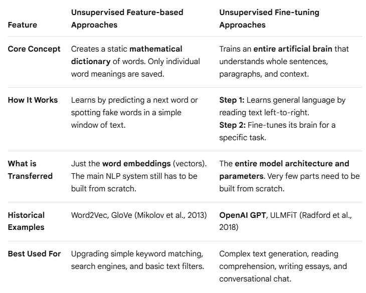
What are the two Transfer Learning Strategies in NLP?
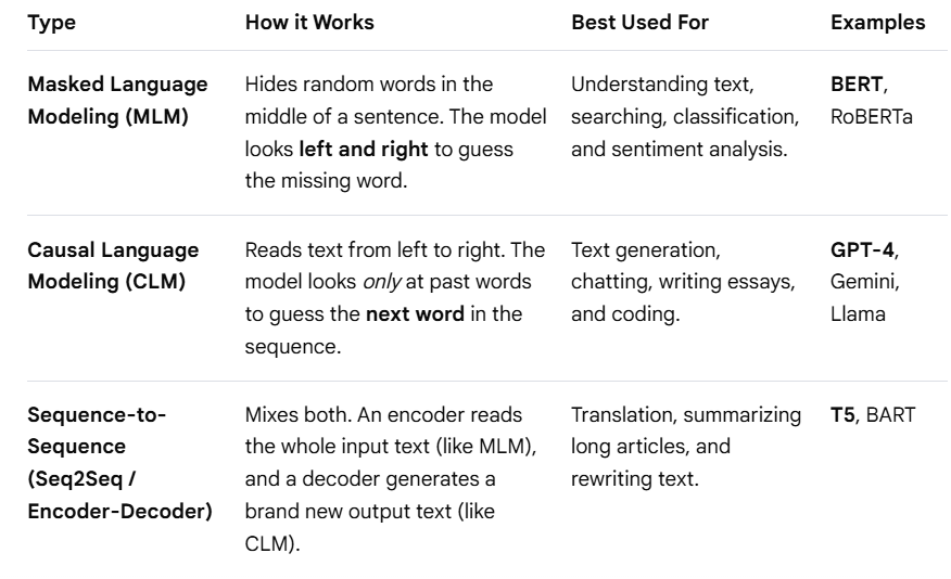
What is Language Model Pre-training Objective?
It is a specific method used to teach an AI how human language works before it is customized for a specific task. Here are the 3 main pre-training objectives, which dive into the details of pre-training and tells how the model learns to understand human language and relationships between words and phrases:
Data Preprocessing
BERT’s input isn’t just a token sequence — it’s built to represent either one sentence or a pair of sentences unambiguously in a single sequence, because the NSP (Next Sentence Prediction) task needs two sentences at once. Two things make this work: a [SEP] token marking where sentence A ends and sentence B begins, and a learned segment embedding added to every token.
Also, [CLS] is a special token is prepended to every input, always in position 0. It doesn’t correspond to any real word. It is used as a summary representation of the entire input sequence, and its final hidden state is used for classification tasks.
So the input to BERT is:
Position embeddings
Segment embeddings: To which sentence the token belongs (A or B)
Token embeddings:
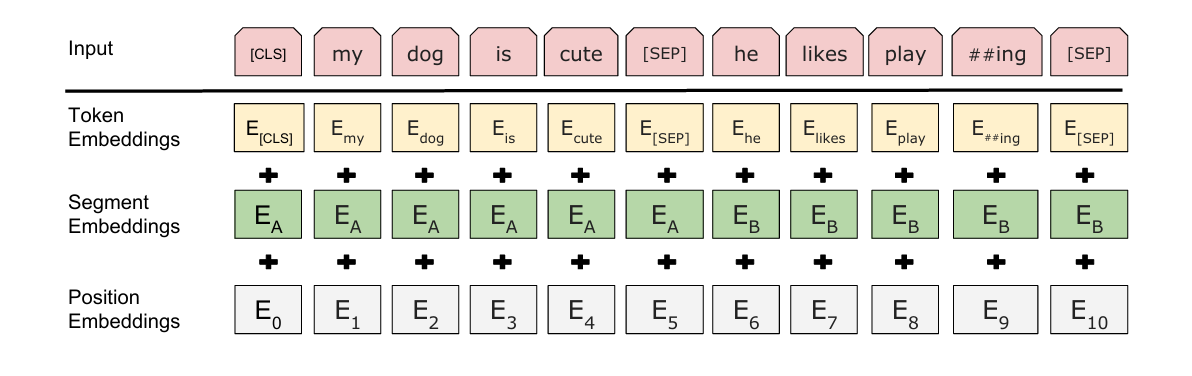
Each token is represented by the sum of the 3 embeddings above.
Adding the vectors preserves their size. In our toy model, each vector has 128 values, so the combined representation also has 128 values. A batch of 32 sequences, each containing 128 tokens, therefore enters the encoder with shape [32, 128, 128].
At this point, a token’s representation does not yet incorporate the surrounding words. That is the job of the encoder layers.
Model Architecture
BERT’s architecture is just the encoder half of the original Transformer, with no changes to the mechanism itself: multi-head self-attention, residual connections, LayerNorm, feed-forward layers, stacked in layers.
Three numbers describe the size of a BERT model:
- L — number of stacked encoder layers
- H — hidden/embedding size, i.e. d_model
- A — number of attention heads
The paper reports two sizes: BERT-BASE (L=12, H=768, A=12, 110M parameters) and BERT-LARGE (L=24, H=1024, A=16, 340M parameters).
The one architectural difference that actually matters: BERT uses bidirectional self-attention — no causal mask — while GPT restricts each token to only attend to tokens before it, via the causal_mask triangle.
Inside one Encoder Layer
After the embeddings are created:
\[ x_i = E_{\text{token}}(t_i) + E_{\text{position}}(i) + E_{\text{segment}}(s_i) \]
The attention mechanism is applied to the input sequence. like this:
\[ Q = XW_Q, \qquad K = XW_K, \qquad V = XW_V \]
\[ \operatorname{Attention}(Q, K, V) = \operatorname{softmax}\left( \frac{QK^{\top}}{\sqrt{d_k}} \right)V \]
Each token produces a query, key, and value vector. Query–key comparisons determine how much weight to give each position. Those weights are then used to combine the value vectors, producing a new representation for each token.
The above is applied in parallel for multiple attention heads, each with its own learned linear projections. The experiment: 128 hidden dimensions divided across 4 heads gives 32 dimensions per head. The outputs of the heads are concatenated and projected again to produce the final output of the multi-head attention layer.
Then we pass through \(W_O\) linear projection.
After that, we have a residual connection and layer normalization:
\[ U = \operatorname{LayerNorm}\left( X + \operatorname{MultiHeadAttention}(X) \right) \]
Another FFN layer.
\[ FFN(U) = \operatorname{ReLU}(UW_1 + b_1)W_2 + b_2 \]
\[ Y = \operatorname{LayerNorm}\left( U + \operatorname{Dropout}\left( FFN(U) \right) \right) \]
This completes one encoder layer. Its output \(Y\) has the same shape as its input \(X\): [batch_size, sequence_length, hidden_size]. What changes is the information in the vectors: each token’s representation now incorporates information from other positions. We pass this output into the next encoder layer, which repeats the same operations with its own learned parameters. Our toy model stacks four such layers.
We concatenate the outputs of all the encoder layers to form a single representation for each token. Then to predict a misssing token, we convert its final contextual vector (The results from the concatenation) into a score for every token in the vocabulary.
\[ Z = X^{(L)}W_{\mathrm{MLM}} + b_{\mathrm{MLM}} \]
This changes the shape from [batch_size, sequence_length, hidden_size] to [batch_size, sequence_length, vocab_size]. The resulting values are called logits. Applying softmax across the vocabulary converts them into probabilities.
Masked Language Modeling (MLM)
When preparing the data for the MLM task, We randomly select approximately 15% of eligible token positions for prediction, excluding special tokens such as [CLS], [SEP], and [PAD].
| Probability | What happens to the input token |
|---|---|
| 80% | Replace it with [MASK] |
| 10% | Replace it with a random vocabulary token |
| 10% | Leave it unchanged |
For example, if “cat” is selected and replaced with [MASK]:
Original:   [CLS]  the  cat     sat  down  [SEP]
Input:      [CLS]  the  [MASK]  sat  down  [SEP]
Target:     ignore ignore cat  ignore ignore ignore
When measuring the loss, we only consider the positions that were selected for prediction, cat in the example above. We take the negative logarithm of the probability assigned to the correct token. Assigning a higher probability to that token gives a smaller loss. We then average over the selected positions.
Training Experiment
We trained a BERT model on a small dataset with approximately 64,000 tokens. The model was trained for 10 epochs with a batch size of 32. Using a 5090RTX GPU, the training took approximately 3 min.
| Epoch | Training loss | Validation loss |
|---|---|---|
| 1 | 7.4333 | 6.9598 |
| 2 | 6.8318 | 6.7418 |
| 3 | 6.7074 | 6.6680 |
| 4 | 6.6273 | 6.6106 |
| 5 | 6.5948 | 6.5776 |
| 6 | 6.5665 | 6.5608 |
| 7 | 6.5402 | 6.5339 |
| 8 | 6.5269 | 6.5224 |
| 9 | 6.5111 | 6.5111 |
| 10 | 6.4975 | 6.4943 |
The model uses four encoder layers, four attention heads, and a hidden size of 128. We reuse AraBERT’s tokenizer, but initialize and train our model weights from scratch. Training loss decreased from 7.4333 to 6.4361, while validation loss decreased from 6.9598 to 6.4485.
Lower loss does not necessarily mean the model can complete sentences sensibly. For example, given “القاهرة هي عاصمة [MASK]”, its highest-ranked prediction was ##ة, rather than the expected answer “مصر”.
Our tokenizer uses WordPiece, so predictions can be word fragments. The ## prefix marks a continuation within a word. Producing fragments is therefore expected, but these particular predictions do not provide useful completions.
Conclusion
This experiment demonstrates the mechanics of the BERT model and how it can be trained on a small dataset. Constructing input embeddings, applying bidirectional attention, and learning to recover selected tokens. It is a simplified implementation, using a small encoder, a linear prediction head, and masked language modeling..
Training code: BERT Toy Notebook.
Comments