Convolutional Neural Networks (CNNs): Intuition, Math, and a Simple Example
In this explainer, we will dive into what a convolutional neural network (CNN) is and explore its main components. We will break down the overall structure of the network, and see the math intuition behind. Then, explore a simple example to see how filters collect important features automatically, and why this makes them so effective for tasks like image recognition and classification.
Let’s get started by looking at the key ideas and building blocks behind CNNs.
We will discuss the following:
Introduction: What is a CNN?
A convolution neural network is a type of artificial neural networks (ANNs), designed to extract features from images and grid-like matrix datasets. A CNN uses a filter to automatically and efficiently extract important features from the grid-like structure data. A filter is a small matrix containing weights that get updated each time the filter slides across the image.
What does this filter collects? It learns which local patterns are important by adjusting its weights values to reduce the error during the training stage. After training, these weights act as indicators, signaling whether certain features or patterns are present in an image.
Key Components of CNNs
A convolution neural network consists of the following:
Filters (kernels) that slide across the input.
Each filter learns to detect a specific local pattern (edges, textures, shapes).
The output is a feature map showing where that pattern appears.
1- Filters (kernels)
These are small matrixs containing weight values. They focus on small regions of the image at a time. Their weights are updating using backpropagation. After training, these filters become specialized in detecting patterns (edges, textures, shapes).
2- Activation function (ReLU)
This function works by keeping useful signals and suppressing weak ones, which enables learning complex patternes. It decides what information is worth passing forward.
3- Pooling Layers
These layers are used to reduce the spacial size (width and height (dimensions) of the input data) while preserving important features. For example, reducing 32×32 image to 16×16, while trying to keep the most important information. This helps make the network more efficient and less sensitive to small shifts or distortions in the input.
4- Feature Maps
A feature map is the output produced when a filter (kernel) slides over the input data. Each filter map corresponds to one filter, and we said before that each filter is specialized in detecting a spicific feature like edges, therefore each feature map shows the locations and strengths of the features that the filter has learned to recognize.
5- Fully Connected Layers
These layers combine all learned features then make the final decision about the image. If its a classification task, then this layer will decide-based on the colleced features- to which class the image belongs.
CNNs Math
1- Convolution
Consider a \(5 \times 5\) image where each value represents a pixle intensity. To create a CNN network, we first define a filter size. For example, let’s use a \(3 \times 3\) filter with randomly initialized values.
Mathematically, a filter (or kernel) \(K\) of size \(3 \times 3\) can be represented as:
\[ K = \begin{bmatrix} k_{1,1} & k_{1,2} & k_{1,3} \\ k_{2,1} & k_{2,2} & k_{2,3} \\ k_{3,1} & k_{3,2} & k_{3,3} \end{bmatrix} = \begin{bmatrix} 0.2 & -0.5 & 0.3 \\ -0.1 & 0.4 & 0.7 \\ 0.6 & -0.2 & 0.1 \end{bmatrix} \]
Each \(k_{i,j}\) is a weight, typically initialized with small random values (e.g., sampled from a normal distribution \(\mathcal{N}(0, \sigma^2)\) or a uniform distribution).
Now let’s assume that the input image matrix is defined as follows:
\[ I = \begin{bmatrix} 1 & 2 & 0 & 3 & 1 \\ 4 & 1 & 1 & 0 & 0 \\ 1 & 2 & 2 & 4 & 1 \\ 3 & 0 & 1 & 2 & 3 \\ 2 & 3 & 0 & 1 & 2 \end{bmatrix} \]
Each entry represents the intensity of a pixel in the \(5 \times 5\) image.
Note:
Keep in mind that all images in modern computers are represented as a grid of matrix initensities, see this image as an example:
Image source: researchgate
In Convolution Operation, we slide the kernel matrix over the input image. At each position, the kernerl weights get multiplied by the pixle values in the input image.
The kernel convolution is applied as the folowing:
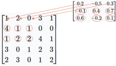
Apply the kernel to the top-left (\(3 \times 3\)) region of the image. We multiply each kernel value by the corresponding image pixel and sum the results:
First region of the image: \[ \begin{bmatrix} 1 & 2 & 0 \\ 4 & 1 & 1 \\ 1 & 2 & 2 \end{bmatrix} \]
Kernel: \[ \begin{bmatrix} 0.2 & -0.5 & 0.3 \\ -0.1 & 0.4 & 0.7 \\ 0.6 & -0.2 & 0.1 \end{bmatrix} \]
Multiply element-wise and sum: \[ \begin{align*} & (1 \times 0.2) + (2 \times -0.5) + (0 \times 0.3) \\ + & (4 \times -0.1) + (1 \times 0.4) + (1 \times 0.7) \\ + & (1 \times 0.6) + (2 \times -0.2) + (2 \times 0.1) \\ = & 0.2 + (-1.0) + 0 \\ + & (-0.4) + 0.4 + 0.7 \\ + & 0.6 + (-0.4) + 0.2 \\ = & (0.2 - 1.0) + (-0.4 + 0.4 + 0.7) + (0.6 - 0.4 + 0.2) \\ = & (-0.8) + (0.7) + (0.4) \\ = & 0.3 \end{align*} \]
So, the output value at the top-left position of the feature map is 0.3.
Then, we move the kernel one position to the right and repeat the process for the next \(3 \times 3\) region of the image:
\[ \begin{bmatrix} 2 & 0 & 3 \\ 1 & 1 & 0 \\ 2 & 2 & 4 \end{bmatrix} \]
Multiply element-wise with the kernel and sum,
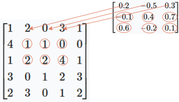
the output value at this position of the feature map is 2.8.
You continue this process, sliding the kernel across the entire image, to fill out the full feature map.
The result (The feature map) is found by sliding the \(3 \times 3\) kernel over the \(5 \times 5\) image. For our example, the full feature map is:
\[ \text{Feature Map} = \begin{bmatrix} 0.3 & 2.8 & 2.2 \\ 0.7 & 1.0 & 2.2 \\ 2.2 & 0.2 & 2.6 \end{bmatrix} \]
Each value is computed by applying the kernel to the corresponding \(3 \times 3\) region of the input image.
2- Applying an Activation Function (ReLU)
We mentioned in the previous section that activation functions are used to that keep useful signals and suppress weak ones, this allows the model to learn complex patterns. Relu works by removing negative signals, and keeping only positive ones.
Applying the ReLU activation function to the feature map means replacing all negative values with zero.
\[ \text{ReLU}(x) = \max(0, x) \]
Applying ReLU to our feature map:
\[ \begin{bmatrix} 0.3 & 2.8 & 2.2 \\ 0.7 & 1.0 & 2.2 \\ 2.2 & 0.2 & 2.6 \end{bmatrix} \;\xrightarrow{\text{ReLU}}\; \begin{bmatrix} 0.3 & 2.8 & 2.2 \\ 0.7 & 1.0 & 2.2 \\ 2.2 & 0.2 & 2.6 \end{bmatrix} \]
In this case, all values are already non-negative, so the feature map remains the same after applying ReLU.
3- Pooling (e.g., Max Pooling)
Pooling layers are used to reduce the spatial dimensions of the feature map while preserving important features. The most common type is max pooling, which takes the maximum value from each region.
When applying a \(2 \times 2\) max pooling operation to our \(3 \times 3\) feature map, we slide a \(2 \times 2\) window over the feature map (stride 1), and for each window, we take the maximum value:
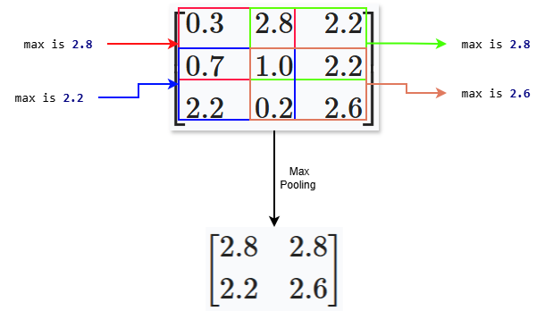
This smaller matrix keeps the most important activations and reduces the amount of data passed to the next layer.
4- Fully Connected Layer
After the max polling, we pass the information to a fully connected layer, a layer with stacked neurons connected to every input from the previous layer. In the pooled feature map, we got a matrix, so we should first flatten the matrix into a one-dimensional vector.This vector contains all the important features extracted by the convolution and pooling layers.
The fully connected (dense) layer then takes this vector and learns to combine these features to make the final prediction.
Mathematically, the fully connected layer performs a matrix multiplication between the flattened input vector and a weight matrix, adds a bias, and applies an activation function (like softmax for classification):
\[ \text{output} = \text{softmax}(W \cdot x + b) \]
Where:
\(x\) is the flattened feature vector (The results from the pooling layer),
\(W\) is the weight matrix,
\(b\) is the bias vector.
After pooling, our feature map is:
\[ P = \begin{bmatrix} 2.8 & 2.8 \\ 2.2 & 2.6 \end{bmatrix} \]
First, flatten this matrix into a vector:
\[ x = \begin{bmatrix} 2.8 \\ 2.8 \\ 2.2 \\ 2.6 \end{bmatrix} \]
Assume the fully connected layer has 2 neurons, thus the weights defined as follows:
\[ W = \begin{bmatrix} w_{1,1} & w_{1,2} & w_{1,3} & w_{1,4} \\ w_{2,1} & w_{2,2} & w_{2,3} & w_{2,4} \end{bmatrix} \]
and bias:
\[ b = \begin{bmatrix} b_1 \\ b_2 \end{bmatrix} \]
The output is:
\[ \text{output} = W \cdot x + b \]
Or, written out:
\[ \begin{bmatrix} w_{1,1} & w_{1,2} & w_{1,3} & w_{1,4} \\ w_{2,1} & w_{2,2} & w_{2,3} & w_{2,4} \end{bmatrix} \begin{bmatrix} 2.8 \\ 2.8 \\ 2.2 \\ 2.6 \end{bmatrix} + \begin{bmatrix} b_1 \\ b_2 \end{bmatrix} = \begin{bmatrix} w_{1,1} \cdot 2.8 + w_{1,2} \cdot 2.8 + w_{1,3} \cdot 2.2 + w_{1,4} \cdot 2.6 + b_1 \\ w_{2,1} \cdot 2.8 + w_{2,2} \cdot 2.8 + w_{2,3} \cdot 2.2 + w_{2,4} \cdot 2.6 + b_2 \end{bmatrix} \]
The network will learn by adjusting its weights and bias values to reduce the loss.
5- Loss Function and Learning
A loss function is used to measure how well the network’s prediction matches the true labels. This is done using a loss function.
During training, the network uses this loss value to adjust its weights and biases through a process called backpropagation. The goal is to minimize the loss, so the network’s predictions become more accurate over time.
This completes the mathematical flow of a CNN: from input image, through convolution, activation, pooling, fully connected layers, and finally to loss and learning.
For more details on loss, refer to this explainer:
Loss Functions
CNNs Code
Create an image of the number 2
Now define the kernel and the feature map to store the output of the covolution, then pass the kernel over the image to get the feature map output:
The feature map will be 8x8 because the kernel is \(3 \times 3\) and the image is \(10 \times 10\), becasue the possible positions along each dimension is (10 - 3 + 1) = 8
Notice how each kernel detects different patterns in the image. We see that each feature map highlights different fratures in the original image of the digit 2.
Apply an Activation Function (ReLU)
Now we pass the above results to an activation function (ReLU):
Notice the effect of ReLU, it shutdown all negative signals and set them to zero (Black box). Each kernel is a pattern detector, applying the kernel to the image means extracting those patternes. If the pattern found, then the return is positive, else it is negative. ReLU suppress all negative signal to zero and only keeps the positive ones.
Pooling (Max Pooling)
In a 2x2 max pooling, we only keeps the largest value from each 2x2 block, we keep the strongest activations. This operation compresses the feature map and reduces its spatial dimensions, making the network more efficient and less sensitive to small shifts or distortions in the input. By keeping only the strongest features using max pooling, we force the model to focus only to the most important features.
The next steps are applying the above to an activation function depending on the task. If the task is classification, then we use softmax(), which will give a probability for each class. For example, it will output the probability of the image being a number 1 or 2 or 3 and so on. Then a loss function is used to measure how well the predicted probabilities match the true class labels. For classification tasks, the most common loss function is cross-entropy loss.
During training, the network uses this loss value to update its weights and biases through backpropagation and gradient descent.
Summary
We introduced CNNs and there components, and build a mathematical foundation of each part of the network. Starting with kernels and demonstrated how they extract features from input images through convolution. Then, introduced activation and pooling and saw how these two steps help the model find the most important features in the image. Finally, connecting these concepts to a fully connected layer, illustrating how the network combines extracted features to make predictions.
Understanding these fundamental ideas provides a strong foundation for further study and practical application of CNNs in computer vision and beyond.
Comments