GPT: Stripping the Encoder Away
In this explainer, we will dive into the architecture of the GPT model, which is a type of transformer model. After goinig through the encoder-decoder architecture, we will see how the GPT model is a decoder-only architecture. We will try to explore the math intuition behind it. Finally, we’ll present a simple code example to demonstrate how the network works in practice.
We will discuss the following:
Introduction
The encoder-decoder architecture works with paired data; english sentences matched to their Arabic translations. Someone had to sit down and label every single training example: this input maps to this output.
GPT asks a different question: what if there’s no source sentence to translate at all — just text to continue?
The training data for GPT is just raw text, with no labels at all. The model is trained to predict the next token in a sequence, given all the previous tokens. This is much simpler and can be done with any text corpus, without the need for human labeling.
This is called self-supervised learning, and it’s the idea GPT is built entirely around. Instead of learning a mapping between two languages, GPT learns to predict the next token in a sequence, over and over, across as much raw text as you can feed it.
For this the architecture of GPT is a decoder-only architecture, making the training much simpler and faster. The encoder is stripped away, and the decoder is left to do all the work. The decoder is a stack of transformer blocks, each with a multi-head self-attention layer, a feed-forward neural network, and layer normalization.
Data Preprocessing
The GPT’s data is a raw text corpus, we can pull Arabic Wikipedia, then a preprocessing step is applied to tokenize the text and shape it into fixed-size training examples.
Tokenization: byte-level BPE, not word-level.
We used byte-level Byte-Pair Encoding (BPE) instead — the same family of tokenizer GPT-1/2 use. Rather than mapping whole words to ids, BPE learns to represent text as a sequence of smaller, frequently-reused subword pieces.
Take the Arabic word العلم (“the knowledge”). Rather than reserving one vocabulary slot for that exact word, the tokenizer we trained represents it as two smaller pieces:
العلم → "الع" + "لم"
Meanwhile, a very common word like هو (“he/it is”) gets its own single token, because it appears often enough in the training text to earn one outright. The tokenizer isn’t choosing arbitrarily — during training it repeatedly merges whichever character sequences occur most frequently in the corpus into single tokens, and falls back to smaller pieces for anything rarer. That’s what “frequently-reused” means in practice: a piece like لم shows up inside dozens of different words, so learning one good representation for it is far more efficient than learning a separate, isolated one for every whole word it happens to appear in.
A nice side effect for a morphologically rich language like Arabic: common prefixes, suffixes, and roots become their own reusable tokens, shared across thousands of different words, instead of each whole word needing its own dedicated vocabulary slot.
Shaping the data: one long stream, chunked into fixed-length blocks.
To make this concrete, imagine a tiny corpus that’s already been tokenized into this single stream of 13 token ids:
[5, 12, 7, 3, 9, 14, 2, 8, 6, 11, 1, 15, 4]
With a (small, illustrative) block size of 4 tokens — the real pipeline uses 128 — we slice off non-overlapping 5-token windows (4 + 1, since each block needs one extra token to shift into):
Block 1: [5, 12, 7, 3, 9] - x = [5, 12, 7, 3] - y = [12, 7, 3, 9]
Block 2: [14, 2, 8, 6, 11] - x = [14, 2, 8, 6] - y = [2, 8, 6, 11]
Notice y is just x shifted one position to the right — at every position, the target is simply “the token that actually comes next.” That’s the entire training signal for language modeling.
In the real pipeline this same process runs over the full 6.67-million-token corpus with 129-token blocks (128 for x, shifted by one for y), producing 52,076 training examples with nothing padded, ever.
Model Architecture
Single GPT Block
For the architecture, we only have the decoder part of the transformer. Containing self-attention mechanism itself — Query, Key, Value, the scaled dot product, multi-head attention, residual connections and LayerNorm. Also, we don’t have the cross-attention mechanism, since we don’t have an encoder to attend to.
We start with the input embeddings, which are the token embeddings and positional embeddings summed together.
If we have a batch of 32 sequences, each of length 128 tokens, and we set the embedding dimension to 128, meaning each token is represented by a 128-dimensional vector, then the input embeddings will have the shape of (32, 128, 128).
Below is a diagram of the first step in the GPT architecture, where we take the input embeddings and split them into multiple heads (4 heads in this case), each with a dimension of 32 (128 / 4). Each head will then perform self-attention independently, allowing the model to capture different aspects of the input sequence.

Now below is a diagram of what is happening inside each head. We take the input embeddings and project them into three different spaces: Query, Key, and Value.
The W_Q, W_K, and W_V are learnable weight matrices that transform the input embeddings into the Query, Key, and Value representations. We get the scores using this formula: \[ \text{scores} = \frac{QK^T}{\sqrt{d_k}} \]
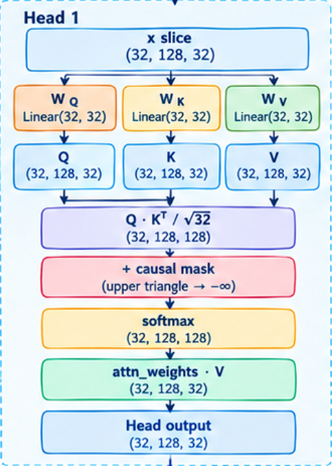
The the scores are then masked using a causal mask, which blocks out any key position that comes after the query position. This is done to ensure that the model only attends to previous tokens in the sequence, and not future tokens.
Then we apply the softmax function to the masked scores to get the attention weights. And finally, we multiply the attention weights with the Value vectors to get the output of the head.
Apply the above process to all heads, and then concatenate the outputs of all heads together. This is done to allow the model to capture different aspects of the input sequence.
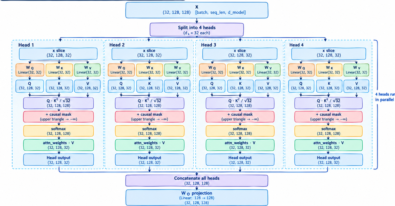
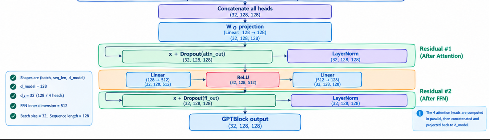
Then after attention and having the results of all heads concatenated, we apply a linear transformation W_O to the concatenated output, then a residual layer followed by a feed forward layer, and finally another residual layer. The feed forward layer is a simple two-layer neural network with a ReLU activation function in between.
Stacking GPT Blocks
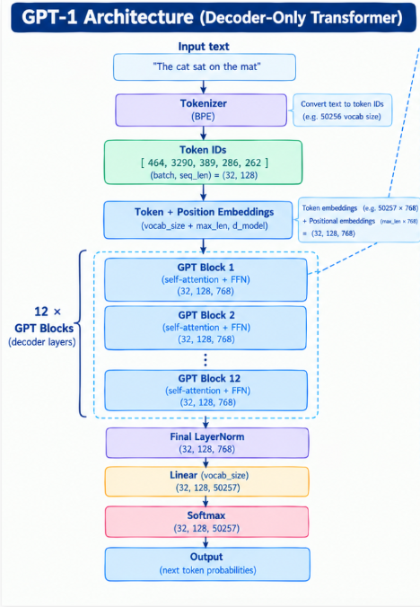
A single GPTBlock refines the token representations once. To capture the kind of long-range structure real language needs, we stack several of these blocks one after another — the output of block 1 becomes the input to block 2, and so on.
In our build, we stack 4 identical GPTBlocks (num_layers=4) — identical in structure, not in weights. Each block has its own independently-learned W_Q, W_K, W_V, W_O, and feed-forward parameters. The first block sees only the raw token embeddings, while the last block sees representations that have already been refined three times over.
Stacking allow richer representations to emerge, and the model to capture more complex patterns in the data.
Training Experiment
We have trained a small GPT model on a small Arabic Wikipedia dataset.The training procedure and model architecture are implemented in the GPT Toy Notebook.
Comments