LSTM Networks: Intuition, Math, and Code
Vanilla RNNs struggle to learn from long sequences — gradients either vanish or explode as they travel back through time, so the network effectively forgets anything more than a few steps back. Long Short-Term Memory (LSTM) networks were designed specifically to fix this.
In this explainer we build up the LSTM from scratch: first the intuition, then the full forward-pass equations, then backpropagation through time (BPTT), and finally a clean code implementation.
We will discuss the following:
Introduction
RNNs contributed to machine learning in a big way and were able to solve tasks that traditional neural networks simply couldn’t, such as predicting the next word in a sentence, translating text, and generating characters one by one. But as sequences start to become longer and longer, RNNs performance starts to decrease, and they strat to forget informations from the begining of the sequence. For example, if we have a long sequence of words from a paragraph, where at the start it mentions “Ahmed, who grew up in Cairo and studied engineering for many years…” and then fifty words later asks the model to complete “Ahmed works as an ___“, a vanilla RNN has likely already lost the word engineering by that point.
LSTM are capable of learning long-term dependencies, and can remember information for long periods of time.
Forward Pass
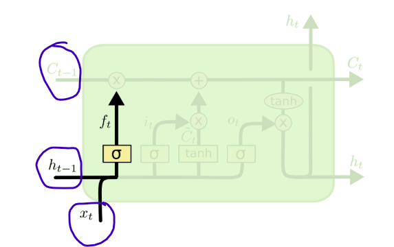
We start with the big picture, each LSTM cell recieves 3 inputs:
\(x_t\) — the current input (e.g. the current character or word)
\(h_{t-1}\) — the hidden state from the previous timestep (short-term memory)
\(c_{t-1}\) — the cell state from the previous timestep (long-term memory)
LSTM diagrams adapted from Christopher Olah’s Understanding LSTM Networks.
Why we need both \(h_t\) and \(c_t\) ?
The \(c_t\) is the memory storage that hold long-term dependencies and information.
The \(h_t\) holds the current information related to the current time step. It is a filtered version of \(c_t\) that exposes only selected information from the memory storage. (Short-term memory)
The main steps in each LSTM cell:
Forget → forget gate \(f_t\) — a number between 0 and 1 for each memory slot. 0 means erase it, 1 means keep it.
Write → input gate \(i_t\) + candidate \(\tilde{c}_t\) — first decide how much to write, then decide what to write.
Update memory → \(c_t = f_t \odot c_{t-1} + i_t \odot \tilde{c}_t\) — old memory scaled by forget, plus new info scaled by input gate.
Expose → output gate \(o_t\) → \(h_t = o_t \odot \tanh(c_t)\) — decide what slice of the memory to broadcast.
Forget gate: In this gate, the model decides what information to throw away from the previous cell state \(c_{t-1}\). The function is: \[ f_t = \sigma(W_f \cdot [h_{t-1}, x_t] + b_f)\]
Where:
\(W_f\) is the weight matrix for the forget gate
\(b_f\) is the bias for the forget gate
\(\sigma\) is the sigmoid activation function, which squashes the output to be between 0 and 1. This allows the model to decide how much of each piece of information to keep (1) or forget (0).
Input gate: In this gate, the model decides what new information to store in the cell state.
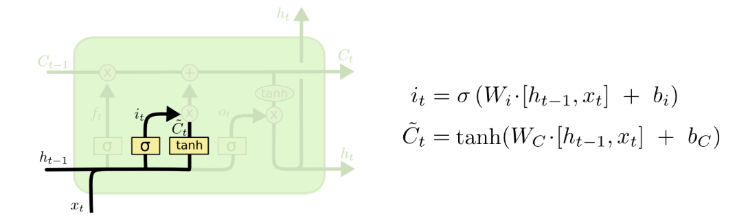
LSTM diagrams adapted from Christopher Olah’s Understanding LSTM Networks.
The input gate has two parts:
Input gate layer \(i_t\) : this layer decides which values from the input to update. The sigmoid function outputs a number between 0 and 1 for each value of the cell state \(C_{t-1}\) to determine how much of each value to update. \[ i_t = \sigma(W_i \cdot [h_{t-1}, x_t] + b_i)\]
Candidate values \(\tilde{c}_t\): this layer creates a vector of new candidate values that could be added to the cell state; the new information the cell wants to add to memory. The \(\tanh\) function squashes the values to be between -1 and 1.
\[\tilde{c}_t = \tanh(W_c \cdot [h_{t-1}, x_t] + b_c)\]
So in this step, the model decides both how much to update (input gate) and what to update (candidate values).
Update cell state: Now we have the forget gate \(f_t\), the input gate \(i_t\), and the candidate values \(\tilde{c}_t\). We can now update the cell state \(c_t\) using the following equation: \[c_t = f_t \odot c_{t-1} + i_t \odot \tilde{c}_t\]
The equation forgets the old cell state \(c_{t-1}\) by multiplying it with the forget gate \(f_t\), and then adds the new candidate values \(\tilde{c}_t\) scaled by how much we decided to update (input gate \(i_t\)).
Output gate: Finally, the output gate decides what to output based on the cell state. It uses the following equations: \[o_t = \sigma(W_o \cdot [h_{t-1}, x_t] + b_o)\] \[h_t = o_t \odot \tanh(c_t)\]
The output gate \(o_t\) decides which parts of the cell state to expose as the hidden state \(h_t\); using a sigmoiod (0 to 1) to filter the cell state. Then \(\tanh\) is applied to the cell state \(c_t\) to squash the values between -1 and 1, and finally the output gate \(o_t\) decides which parts of that to actually output as the hidden state \(h_t\).
Code Example
Here is an experiment where we train an LSTM to generate Arabic text character by character. The notebook contains a step by step walkthrough of the code, and what does each line do. You can find the notebook here
Track cell states
We can also track the cell states as we feed in a sequence of characters, and visualize how the values in the cell state change over time. Each cell in the \(c_t\) vector, if the vector size is 128 for each time step, then we have 128 “cells” that can each store a different piece of information.
After defining our model with this:
CharGenerator(
  (embed): Embedding(47, 32)
  (lstm): LSTM(32, 128, batch_first=True)
  (fc): Linear(in_features=128, out_features=47, bias=True)
)
We can feed this sample text into the model: text = 'الكتاب الذي قرأته كان رائعاً جداً والقصة مشوقة'
Then track the cell states as we feed in each character one by one. The text has 46 characters, and the cell state vector has 128 cells, so we end up with a matrix of shape (46, 128), for each character there are 128 cells that can each store a different piece of information. torch.Size([46, 128])
Finally we pick one cell index cell_idx = 29 and visualize how the value in that cell changes as we feed in each character. We can print a bar for each character, where the length of the bar corresponds to the value in that cell, longer bars mean the cell is more “activated” for that character.
Here is the result for cell index 29:
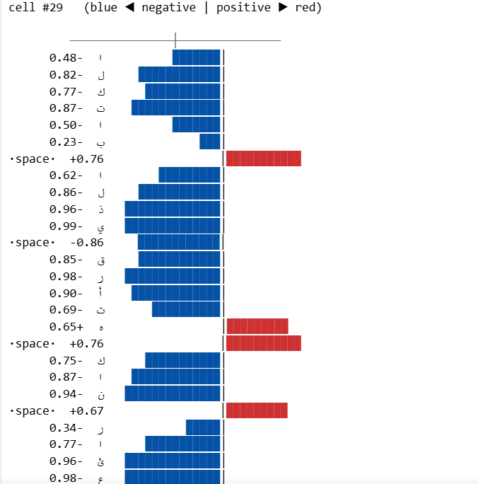
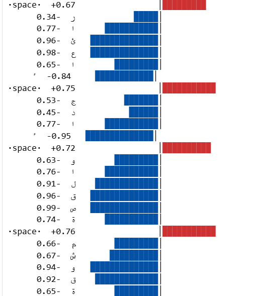
The above shows how the cell #29 reacts to each character in the input text. We can see that it reacts strongly to the space character. Therefore we can say that this cell has learned to detect spaces in the text, and it is likely being used by the model to help it understand word boundaries.
Summary
LSTM is an improvemnt of the vanilla RNN, it is more powerful and can learn long-term dependencies. It has multiple gates that control the flow of information, allowing it to decide what to remember, what to forget, and what to output at each time step. We perfomed a simple training of an LSTM to generate Arabic text, using the same data and training loop as the vanilla RNN, and we got much better results. We also tracked the cell states and visualized how they react to different characters, observing that some cells learn to detect specific features like spaces.
Comments