Recurrent Neural Networks (RNNs)
In this explainer, we will dive into what a recurrent neural network (RNN) is and explore its main components. We will go over the structure of the network, and try to explore the math intuition behind it. Finally, we’ll present a simple code example to demonstrate how the network works in practice.
We will discuss the following:
Introduction: What is an RNN network?
RNN is a type of a neural network designed to process sequential data. It keeps a memory of past inputs and use it along with the current input to predict the new output. Unlike the feedforward networks, RNNs has a loop that allows information from the past to influence the present. For example, think of reading a sentance or a long paragraph, in order to understand the current word, you need to remember the previous words. RNN works the same by keeping a hidden state (memory) of past words to predict the next.
Why not using feedforward networks for sequence learning tasks?
Feedforward neural networks (FFNNs) require inputs of a fixed size, while text and audio can have variable lengths.
FFNNs need separate parameters for each input position, which leads to a large number of parameters when modeling sequences, especially long ones.
A pattern learned in FFNNs cannot be reused at another position. The pattern
A → B → Cis considered different in these two sequences:X A B C YandD D A B C D.
Key Components of RNNs
RNNs take a sequence of inputs: words in a sentance, sensor readings over time,
Hidden state (h_t), it stores information from previous time steps. And at each time step, it updates this memory using the current input and the previous hidden state.
Weights are shared across time (The same network is reused at every time step).
The output (y_t) can produce an output at every time step or only in the final output.
Three shared weight matrices: input-to-hidden, hidden-to-hidden (recurrent), and hidden-to-output, applied at every time step.
Activation function, and the training uses Backpropagation Through Time (BPTT).
RNNs Math
For each stage in the RRN network, there is the following components:
• \(x^{(t)}\): input at time step \(t\)
• \(a^{(t)}\): hidden state (activation) at time step \(t\)
• \(y^{(t)}\): output at time step \(t\)
• \(a^{(0)}\): initial hidden state
Here is the architecture of a traditional RNN:
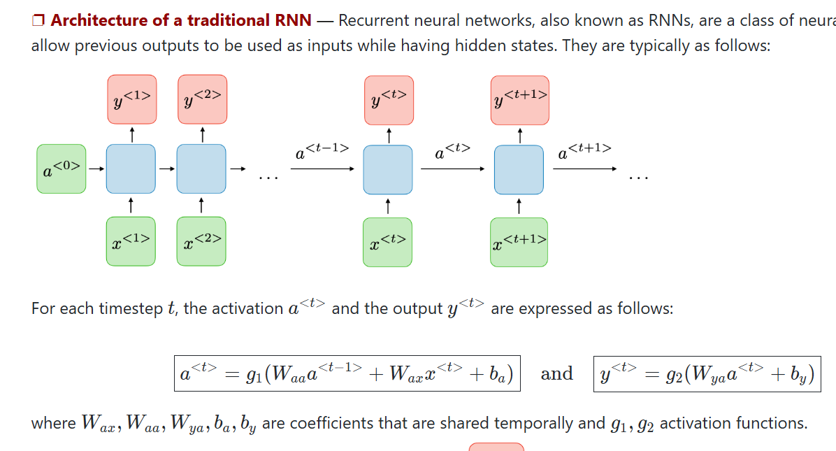
Image credit: Stanford CS-230 Cheatsheet - Recurrent Neural Networks
Let’s focus on the first block (stage) of the network. We need an initial hidden state \(a^{(0)}\), and an initial input value \(x^{(1)}\). These will give us the first hiddent state \(a^{(1)}\). Here is the equation for finding the first hidden state:
\[a^{(1)} = g_1(W_{aa}a^{(1-1)} + W_{ax}x^{(1)} + b_a)\]
where:
- \(W_{aa}\): weight matrix for the hidden-to-hidden connection (recurrent weights)
- \(W_{ax}\): weight matrix for the input-to-hidden connection
- \(b_a\): bias term for the hidden state
- \(g_1\): activation function (typically tanh or ReLU)
For the output at that time step (t), we use the following: \[y^{(1)} = g_2(W_{ya}a^{(1)} + b_y)\]
where:
- \(W_{ya}\): weight matrix for the hidden-to-output connection
- \(b_y\): bias term for the output
- \(g_2\): activation function for the output (typically softmax for classification or linear for regression)
For the loss function, there are two types depending on the type of learning we are using RNN for:
| Architecture Type | Used In | Loss Function |
|---|---|---|
| Many-to-Many (per-step loss) | • Language modeling • Sequence labeling • Time-series forecasting |
Per-step loss: \(\ell^{(t)} = \mathcal{L}(y^{(t)}, \hat{y}^{(t)})\) Examples: • Cross-entropy (classification) • Mean squared error (regression) Total sequence loss: \(\mathcal{L} = \sum_{t=1}^{T} \ell^{(t)}\) |
| Many-to-One (Loss only at the final time step) | • Sentiment analysis • Sequence classification |
\(\mathcal{L} = \mathcal{L}(y^{(T)}, \hat{y})\) The hidden state \(a^{(T)}\) summarizes the entire sequence. |
How is the model trained?
- Backpropagation Through Time (BPTT): where the RNN is unrolled across time steps, then gradients propagated backward from the last time step to the first.
Remember this
RNNs accept an input vector \(x\) and produce an output vector \(y\). However, this output vector is influenced not only by the current input, but also by the entire history of previous input.[karpathy.github.io]
Comments