Simple Math for Recurrent Neural Networks (RNNs)
In this explainer, we will dive into the math behind recurrent neural networks (RNNs) and explore how they process sequential data. We will work on a simple sequance prediction task, where the RNN will learn to predict the next character in the word “hello”. We will go through the forward pass, compute the loss, and then perform the backward pass to update the weights. Finally, convert the math to code to see how it works in practice.
We will discuss the following:
Data preprocessing
To start with, we will break down the word “hello” into its individual characters and convert each character into a one-hot vector. The input sequence will be “h”, “e”, “l”, “l” and the target sequence will be “e”, “l”, “l”, “o”.
Assigning indices to each character:
‘h’: 0
‘e’: 1
‘l’: 2
‘o’: 3
The input sequence “hello” will be represented as:
“h” → [1, 0, 0, 0]
“e” → [0, 1, 0, 0]
“l” → [0, 0, 1, 0]
“l” → [0, 0, 1, 0]
“o” → [0, 0, 0, 1]
The target sequence “elloh” will be represented as:
“e” → 1
“l” → 2
“l” → 2
“o” → 3
Forward Pass
For starting with RNN, we will define the following components: - Input sequence: “hello” (we will convert each character to a one-hot vector) - Target sequence: “elloh” (the next character for each input character) - Hidden state size: 3 (for simplicity) - Weights
Here is the general idea of an RNN network:
We have a sequance of inputs that we will process each one at each time step. And at each time step, we will update the hidden state using the current input and the previous hidden state. So we have:
- Input sequence: \(x^{(1)}, x^{(2)}, ..., x^{(T)}\)
- Hidden states: \(h^{(1)}, h^{(2)}, ..., h^{(T)}\)
- Output sequence: \(y^{(1)}, y^{(2)}, ..., y^{(T)}\)
Here is a simple graphical representation of the RNN:
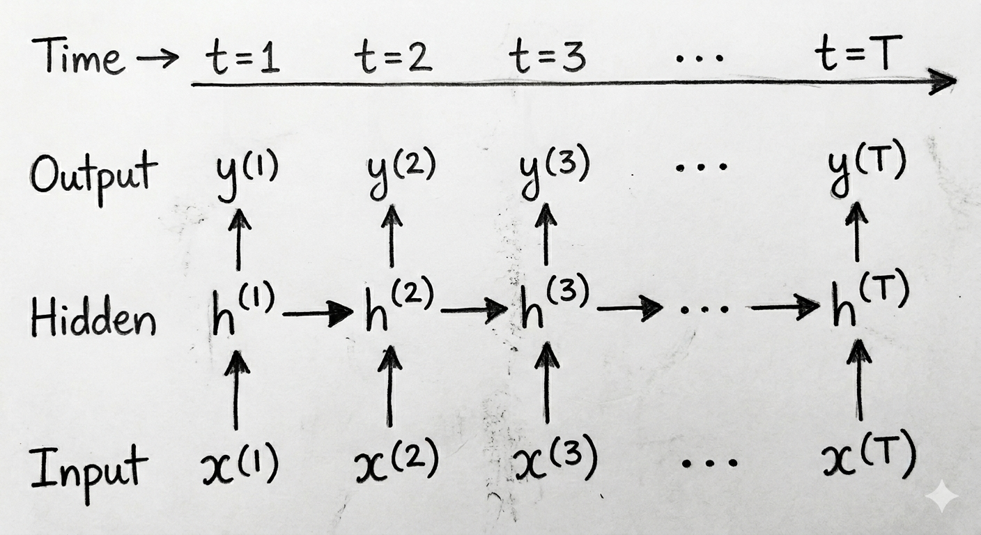
For the sequance “hello”, it has 5 characters, so we will have 5 time steps. The input “h” will be processed at time step 1 and its output will be used to predict “e”. The input “e” will be processed at time step 2 and its output will be used to predict “l”, and so on.
Let’s focus on the first time step and see what is happening mathematically:
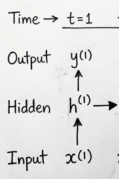
The above image shows the input vector \(x^{(1)}\), the hidden state \(h^{(1)}\), and the output \(y^{(1)}\). Each arrow represents a matrix multiplication with the corresponding weights. Here is a breakdown of the arrows:
The arrow from \(x^{(1)}\) to \(h^{(1)}\) represents the input-to-hidden weights (\(W_{xh}\)).
The arrow from \(h^{(0)}\) (initial hidden state, not appearing in the image) to \(h^{(1)}\) represents the hidden-to-hidden weights (\(W_{hh}\)).
The arrow from \(h^{(1)}\) to \(y^{(1)}\) represents the hidden-to-output weights (\(W_{hy}\)).
The mathematical equations for the forward pass at time step 1 are as follows: \[h^{(1)} = \tanh(W_{xh}x^{(1)} + W_{hh}h^{(0)} + b_h)\] \[y^{(1)} = W_{hy}h^{(1)} + b_y\]
Where:
\(W_{xh}\) is the input-to-hidden weight matrix.
\(W_{hh}\) is the hidden-to-hidden weight matrix.
\(W_{hy}\) is the hidden-to-output weight matrix.
\(b_h\) is the hidden state bias vector.
\(b_y\) is the output state bias vector.
Then we take the output \(y^{(1)}\) and apply a softmax function to get the probabilities, these indicate the model’s confidence about the next character being “e”, “l”, “o”, etc.
Calculated as follows: \[p^{(1)} = \text{softmax}(y^{(1)})\]
Where \(p^{(1)}\) is the probability distribution over the possible next characters.
Now plug in the values:
\[x^{(1)} = [0, 1, 0, 0]\]
\[h^{(0)} = [0, 0, 0]\]
\[W_{xh} = \begin{bmatrix} 0.1 & 0.2 & 0.3 \\ 0.4 & 0.5 & 0.6 \\ 0.7 & 0.8 & 0.9 \\ 1.0 & 1.1 & 1.2 \end{bmatrix}\]
\[W_{hh} = \begin{bmatrix} 0.1 & 0.2 & 0.3 \\ 0.4 & 0.5 & 0.6 \\ 0.7 & 0.8 & 0.9 \end{bmatrix}\] \[W_{hy} = \begin{bmatrix} 0.1 & 0.2 & 0.3 \\ 0.4 & 0.5 & 0.6 \\ 0.7 & 0.8 & 0.9 \\ 1.0 & 1.1 & 1.2 \end{bmatrix}\] \[b_h = [0.1, 0.2, 0.3]\] \[b_y = [0.1, 0.2, 0.3, 0.4]\]
Calculating the hidden state \(h^{(1)}\): \[h^{(1)} = \tanh(x^{(1)}W_{xh} + W_{hh}h^{(0)} + b_h)\] \[= \tanh\left(\begin{bmatrix} 0 \\ 1 \\ 0 \\ 0 \end{bmatrix} \begin{bmatrix} 0.1 & 0.2 & 0.3 \\ 0.4 & 0.5 & 0.6 \\ 0.7 & 0.8 & 0.9 \\ 1.0 & 1.1 & 1.2 \end{bmatrix} + \begin{bmatrix} 0.1 & 0.2 & 0.3 \\ 0.4 & 0.5 & 0.6 \\ 0.7 & 0.8 & 0.9 \end{bmatrix} \begin{bmatrix} 0 \\ 0 \\ 0 \end{bmatrix} + \begin{bmatrix} 0.1 \\ 0.2 \\ 0.3 \end{bmatrix}\right)\]
\[= \tanh\left(\begin{bmatrix} 0.5 \\ 0.7 \\ 0.9 \end{bmatrix}\right) = \begin{bmatrix} 0.462 \\ 0.604 \\ 0.716 \end{bmatrix}\]
Calculating the output \(y^{(1)}\): \[y^{(1)} = W_{hy}h^{(1)} + b_y\] \[= \begin{bmatrix} 0.1 & 0.2 & 0.3 \\ 0.4 & 0.5 & 0.6 \\ 0.7 & 0.8 & 0.9 \\ 1.0 & 1.1 & 1.2 \end{bmatrix} \begin{bmatrix} 0.462 \\ 0.604 \\ 0.716 \end{bmatrix} + \begin{bmatrix} 0.1 \\ 0.2 \\ 0.3 \\ 0.4 \end{bmatrix} = \begin{bmatrix} 0.4818 \\ 1.1164 \\ 1.751 \\ 2.3856 \end{bmatrix}\]
Calculating the probabilities \(p^{(1)}\): \[p^{(1)} = \text{softmax}(y^{(1)})\] \[= \text{softmax}\left(\begin{bmatrix} 0.4818 \\ 1.1164 \\ 1.751 \\ 2.3856 \end{bmatrix}\right) = \begin{bmatrix} 0.076 \\ 0.143 \\ 0.270 \\ 0.511 \end{bmatrix}\]
Before moving to the loss calculaion, let’s first understand the choice of dimensions for the weights and hidden state. It is decided based on the input size, hidden state size, and output size.
| Component | Purpose | Shape | Why This Shape? | |
|---|---|---|---|---|
| \(x^{(t)}\) | Input vector at time step \(t\) | \((1 \times 4)\) | Vocabulary/input feature size is 4 | |
| \(h^{(t)}\) | Hidden state (memory) | \((1 \times 3)\) | Hidden layer has 3 neurons | |
| \(y^{(t)}\) | Output logits | \((1 \times 4)\) | Predicting 4 possible output classes |
| Matrix | Purpose | Space Transformation | Shape | Matrix Multiplication |
|---|---|---|---|---|
| \(W_{xh}\) | Input → Hidden | Input space \(\rightarrow\) Hidden space | \((4 \times 3)\) | \((1 \times 4)(4 \times 3) \rightarrow (1 \times 3)\) |
| \(W_{hh}\) | Hidden → Hidden | Hidden space \(\rightarrow\) Hidden space | \((3 \times 3)\) | \((1 \times 3)(3 \times 3) \rightarrow (1 \times 3)\) |
| \(W_{hy}\) | Hidden → Output | Hidden space \(\rightarrow\) Output space | \((3 \times 4)\) | \((1 \times 3)(3 \times 4) \rightarrow (1 \times 4)\) |
Loss Calculation
In the loss calculation step, we will compute the cross-entropy loss, it is simply taking the index of the target character (which is “e” with index 1), then taking the negative log, if the model is confident about the correct class, the loss will be low, and if it is not confident, the loss will be high. As follows: \[L^{(1)} = -\log(p^{(1)}[1])\]
Where \(p^{(1)}[1]\) is the probability assigned to the correct class “e” (index 1) by the model at time step 1. In this case, \(p^{(1)}[1] = 0.143\), so the loss will be:
\[ L^{(1)} = -\log(0.143) \approx 1.94 \]
Why using the negative log?
See the table below, with the correct probability the loss is low, and vice versa:
| Correct Probability | Loss |
|---|---|
| 0.99 | 0.01 |
| 0.9 | 0.10 |
| 0.5 | 0.69 |
| 0.1 | 2.30 |
| 0.01 | 4.60 |
For each time step the loss is calculated, then we sum up the losses across all time steps to get the total loss for the sequence, which is what we will use to update the weights during the backward pass.
Backward Pass
Now that we have calculated the loss, we will perform the backward pass to compute the gradients and update the weights. We need to update the weights \(W_{xh}\), \(W_{hh}\), and \(W_{hy}\) based on the loss we calculated.
Let’s take the example this training sequance:
Input  (X): h  e  l  l
Target (Y): e  l  l  o
We have 4 time steps, so we will have 4 losses: \(L^{(1)}\), \(L^{(2)}\), \(L^{(3)}\), and \(L^{(4)}\).
At timestep 4:
input  = x(4) = "l"
target = y_true(4) = "o"
This time step recieves:
\(h^{(3)}\) from the previous hidden state
\(x^{(4)}\) from the input sequence
To get the backward pass, we need to remember the forward pass equations:
\(h^{(4)} = \tanh(x^{(4)}W_{xh} + h^{(3)}W_{hh} + b_h)\)
\(y^{(4)} = h^{(4)}W_{hy} + b_y\)
\(p^{(4)} = \text{softmax}(y^{(4)}) = p^{(4)} = \begin{bmatrix} 0.076 \\ 0.143 \\ 0.270 \\ 0.511 \end{bmatrix}\)
\(L^{(4)} = -\log(p^{(4)}[3]) = -\log(0.511) \approx 0.67\)
Now we will compute the gradients for the weights. We will start with the output layer and then move backward to the hidden layers.
\[\frac{\partial L^{(4)}}{\partial y^{(4)}} = \frac{\partial L^{(4)}}{\partial p^{(4)}} \cdot \frac{\partial p^{(4)}}{\partial y^{(4)}} = p^{(4)} - y^{(4)} \]
Now backpropagate the error to the hidden layer:
\[ \frac{\partial L^{(4)}}{\partial h^{(4)}} = \frac{\partial L^{(4)}}{\partial y^{(4)}} \cdot \frac{\partial y^{(4)}}{\partial h^{(4)}}\]
We need to find \(\frac{\partial y^{(4)}}{\partial h^{(4)}}\):
\[\frac{\partial y^{(4)}}{\partial h^{(4)}} = W_{hy}^T\]
This from the equation \(y^{(4)} = h^{(4)}W_{hy} + b_y\)
\[ \frac{\partial L^{(4)}}{\partial h^{(4)}} = \frac{\partial L^{(4)}}{\partial y^{(4)}} \cdot W_{hy}^T\]
Also propagate the error through the tanh activation function: \[\frac{\partial L^{(4)}}{\partial h^{(4)}} = \frac{\partial L^{(4)}}{\partial y^{(4)}} \cdot W_{hy}^T \odot (1 - (h^{(4)})^2)\]
Note: The \((1 - (h^{(4)})^2)\) is the derivative of the tanh activation function.
Now the gradient of the loss with respect to the hidden state \(h^{(4)}\) is calculated, we can now compute the gradients for the weights \(W_{hy}\), \(W_{hh}\), and \(W_{xh}\).
\[ \frac{\partial L^{(4)}}{\partial W_{hy}} = {h^{(4)}}^T \cdot \frac{\partial L^{(4)}}{\partial y^{(4)}} \]
\[ \frac{\partial L^{(4)}}{\partial W_{hh}} = {h^{(3)}}^T \cdot \frac{\partial L^{(4)}}{\partial h^{(4)}} \]
\[ \frac{\partial L^{(4)}}{\partial W_{xh}} = {x^{(4)}}^T \cdot \frac{\partial L^{(4)}}{\partial h^{(4)}} \]
| Gradient | Equation | Notes |
|---|---|---|
| \(\frac{\partial L^{(4)}}{\partial y^{(4)}}\) | \(p^{(4)} - y^{(4)}\) | “How wrong was each output probability?” |
| \(\frac{\partial L^{(4)}}{\partial h^{(4)}}\) | \(\frac{\partial L^{(4)}}{\partial y^{(4)}} \cdot W_{hy}^T \odot (1 - (h^{(4)})^2)\) | Output error and memory error |
| \(\frac{\partial L^{(4)}}{\partial W_{hy}}\) | \({h^{(4)}}^T \cdot \frac{\partial L^{(4)}}{\partial y^{(4)}}\) | Output weight gradient |
| \(\frac{\partial L^{(4)}}{\partial W_{hh}}\) | \({h^{(3)}}^T \cdot \frac{\partial L^{(4)}}{\partial h^{(4)}}\) | Recurrent weight gradient |
| \(\frac{\partial L^{(4)}}{\partial W_{xh}}\) | \({x^{(4)}}^T \cdot \frac{\partial L^{(4)}}{\partial h^{(4)}}\) | Input weight gradient |
This is the grenal equations:
| Gradient | General Equation | Why a sum? |
|---|---|---|
| \(\frac{\partial L}{\partial y^{(t)}}\) | \(dy^{(t)} = p^{(t)} - y_{true}^{(t)}\) | Computed independently per time step — no sum needed |
| \(\frac{\partial L}{\partial h^{(t)}}\) | \(dh^{(t)} = dy^{(t)} W_{hy}^T + dh^{(t+1)} W_{hh}^T \odot (1 - (h^{(t+1)})^2)\) | Computed independently per time step — no sum needed |
| \(\frac{\partial L}{\partial W_{hy}}\) | \(\sum_{t=1}^{T} {h^{(t)}}^T dy^{(t)}\) | \(W_{hy}\) is the same matrix used at every time step. Each step \(t\) contributes \({h^{(t)}}^T dy^{(t)}\) to the gradient. We sum them all because every use of \(W_{hy}\) in the forward pass must be accounted for in the backward pass. |
| \(\frac{\partial L}{\partial W_{hh}}\) | \(\sum_{t=1}^{T} {h^{(t-1)}}^T dh^{(t)}\) | Same reason — \(W_{hh}\) is reused at every step. Each step contributes \({h^{(t-1)}}^T dh^{(t)}\). |
| \(\frac{\partial L}{\partial W_{xh}}\) | \(\sum_{t=1}^{T} {x^{(t)}}^T dh^{(t)}\) | Same reason — \(W_{xh}\) is reused at every step. Each step contributes \({x^{(t)}}^T dh^{(t)}\). |
Code Implementation
Now let’s convert the math we have discussed into code.
reference to a the notebook:
Comments