What is Neural Network?
In this explainer we will go through an introductory overview on neural networks. We will try to introduce the overall concept with the genreal math invloved in each part.
We will discuss the following:
Introduction: What is a neural network?
The idea of neural network is inspired by how neurons in the brain work together to process information. The network consists of multiple layers, each layer with multiple neurons. Every neuron in a layer is connected to all the neurons in the previous layer and the next layer, allowing information to flow through the network and enabling it to learn complex patterns from data.
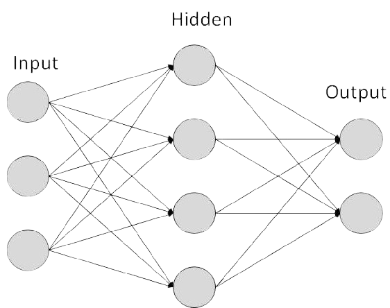
Image credit: almabetter.com
The following section go through a quick overview of each main component of a basic neural network:
Key Components
1- Input layer:
This layer holds the input features \((x_1, x_2, x_3, .....)\). These will go to a series of transformations, they will be added together, multiplied by other vairables (weights), passed through activation functions, and so on. There values will remain unchanged through the training process. If for example the network is learning to predict house prices, the input layer might receive features like the number of rooms, size in square meters, and location score. The network will use these values to learn and give the best prediction for house prices.
2- Hidden layers:
In these layers the core work of learning occur. Each neural connection (the line connecting two neurons) is represented mathematically by a weight \((w)\) value, and finding the best values for these weights is what the learning process is all about. In this layer the network will try to learn the best values of all weights that will give the best house prices prediction.
The number of hidden layers and the neurons in each layer is configured based on the task. Generally, the more complex the problem, the more layers and neurons may be needed to capture patterns in the data.
We can say that each hidden layer consists of:
- Weighs: values representing the connection strength between two neurons.
- Bias: An extra value added to the weighted sum, allowing the neuron to shift the activation function and make the model more flexible.
- Activation Function: A function that introduces non-linearity, helping the network learn complex patterns.
3- Output layer:
In this layer, all previous calculations are combined to produce the network’s prediction. Following the house price prediction, the final layer will produce a single number representing the predicted price. Or if the task is a classification task, then the output will be a list of probabilities.
Forward Pass
Neural networks can become very deep and complex (left image). However, in order to understand the intuition and math behind , we will work on a simple two layers and two neurons network (illustrated on the right):
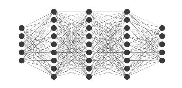 Deep, complex neural network
Image credit:istockphoto.com
 Simple two-layer, two-neuron network
Image credit:victorzhou.com/blog
The main goal of a forward pass is to take the inputs, multiply them by the weights (initial weights if this is the first training step), then get the initial prediction. This is the simplest step in the training process.
Let’s consider the following example:
Suppose we want to predict whether a student will pass an exam (output = 1) or fail (output = 0) based on two features: hours studied and hours of sleep. Here’s how some example data might look:
| Hours Studied | Hours of Sleep | Pass (1) / Fail (0) |
|---|---|---|
| 2 | 5 | 0 |
| 4 | 6 | 0 |
| 6 | 7 | 1 |
| 8 | 8 | 1 |
| 3 | 4 | 0 |
| 7 | 6 | 1 |
The input layer will have two inputs, \(x_1\) for hours studied and \(x_2\) for hours of sleep.
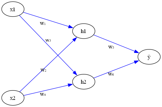
From each node \(x_1\) and \(x_2\) there are two arrows, these represent the weights \(w\), which are the learning parmeters the model will keep adjusting through out the training process.
Intuition: Think of each arrow (weight) as a volume knob that controls how much influence each input has on the next layer. When starting the learning with random values for these weights, the network doesn’t know which inputs are important, so its prediction is far and the error rate is large. As the model learns, it turns these knobs up or down—adjusting the weights, with this the important information will pass and the network will start to get closer to the correct predictions.
Forward Pass: Math Steps
Let’s break down the math for a simple neural network with two inputs (\(x_1\), \(x_2\)), two hidden neurons (\(h_1\), \(h_2\)), and one output (\(\hat{y}\)):
2. Apply the activation function (ReLU):
\[ h_1 = \text{activation}(z_1) \] \[ h_2 = \text{activation}(z_2) \]
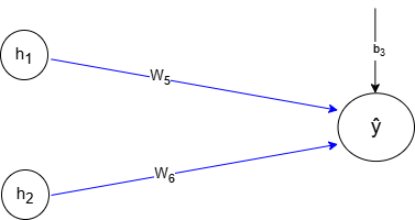
3. Calculate the output neuron’s input:
The output neuron will take the sum of each hidden neuron multiplied by new weight values, plus a bias.
\[ z_3 = w_5 h_1 + w_6 h_2 + b_3 \]
4. Apply the output activation function (sigmoid for binary classification):
\[ \hat{y} = \text{activation}(z_3) \]
………..describe above………..
Forward Pass: Code
Here we turn the above math steps into code, and see what the last nuron will return:
Run the above cell, then run the cell below to see the predicted output: The code will do the following:
Loop through each sample.
Get \(z_1\) and \(z_2\) .
Get \(h\) by passing \(z\) through activation (Relu).
Get \(z_3\)
Pass \(z_3\) through a sigmoid to get \(\hat{y}\)
Each sample representing a student score, we see the network predicts a probability of about 63.3% that the first student will pass the exam. However, the actual outcome for the first student is a fail.
How can we guide the model to adjust its weights to get closer to the correct prediction?
This is where Backpropagation comes in. It is the key algorithm that allows the network to learn from its mistakes.
Backward Pass
The backward pass, or Backpropagation is where the model training occurs. Its core idea is to adjust the weights to get the model predictions closer to the true output results (pass or fail in previous example), here is the main steps in this stage:
Get the error, Using a loss function, calculate how far the model from the true value.
Compute Gradients, how much each weight contributed to the error.
Update each weight and bias in the network to reduce the error (using gradient descent).
Repeat the process for many times (epochs) using many training samples.
What is a loss function?
It is a formula that measures how far off the model’s prediction is from the true value. There are many types of loss functions each designed for a specific task.
For a detailed explanation of loss functions and how to choose the right one for your task, see our Loss Functions explainer.
For our example, we will use the Binary Cross-Entropy loss function because we want the model to predict a binary outcome—whether a student will pass (1) or fail (0) the exam.
it is defined like this:
\[ \text{Loss} = -\frac{1}{n} \sum_{i=1}^{n} \left[ y_i \log(\hat{y}_i) + (1 - y_i) \log(1 - \hat{y}_i) \right] \]
\(\hat{y}_i\): is the predicted probability for sample \(i\).
\(y_i\) is the true value in the training dataset.
\(n\): is the total number of samples in the dataset (how many examples you have).
Let’s see how the loss is calculated for the first sample, where the predicted value is \(\hat{y}_1 = 0.633\) and the true value is \(y_1 = 0\).
The Binary Cross-Entropy loss for one sample is:
\[ \text{Loss}_1 = -\left[ y_1 \log(\hat{y}_1) + (1 - y_1) \log(1 - \hat{y}_1) \right] \]
Plug in the values:
\(y_1 = 0\)
\(\hat{y}_1 = 0.633\)
So, \[ \text{Loss}_1 = -\left[ 0 \cdot \log(0.633) + (1 - 0) \cdot \log(1 - 0.633) \right] \]
\[ = -\left[ 0 + 1 \cdot \log(0.367) \right] \]
\[ = -\log(0.367) \]
\[ \approx -(-1.002) \]
\[ \approx 1.002 \]
So, the loss for this sample is about 1.002.
The next step in this stage is to reduce this error..
Gradient Decent
Gradient descent is the algorithm used to minimize the loss function and improve the prediction. It represent the amount of change that should be applied to the weights in order to reduce the error. In each training step, the algorithm moves the weights slightly in the direction that most reduces the loss.
Choose a loss function: \[ L(w) \]
Compute the gradient: \[ g = \frac{\partial L}{\partial w} \]
Update the parameter:
\[ w_{\text{new}} = w_{\text{old}} - \eta \, g \]
where \(\eta\) is the learning rate (step size).
- Repeat until convergence:
\[ w^{(t+1)} = w^{(t)} - \eta \, \frac{\partial L}{\partial w^{(t)}} \]
Note:
The gradient (or derivative) for each weight is different because it measures how much changing that specific weight will affect the loss. In other words, the gradient tells us the sensitivity of the loss to each weight. We calculate this by taking the derivative of the loss function with respect to each weight using the chain rule in calculas.
Output layer gradients
We have:
\[ \hat{y} = \sigma(z_3), \qquad L = -\left[y \log(\hat{y}) + (1-y)\log(1-\hat{y})\right] \]
We take the derivative of \(L\) with respect to \(z_3\), this tells us how much changing \(z_3\) will affect the loss:
\[ \frac{\partial L}{\partial z_3} = \hat{y} - y \]
The output neuron is:
\[ z_3 = w_5 h_1 + w_6 h_2 + b_3 \]
To get the other gradients, we need to apply the chain rule. This means we move backward from the loss toward each weight, multiplying the gradients along that path, the result is telling how much a change in that weight will affect the loss.
\[ \frac{\partial L}{\partial w_5} = \frac{\partial L}{\partial z_3} \cdot \frac{\partial z_3}{\partial w_5} = (\hat{y} - y)\, h_1 \]
\[ \frac{\partial L}{\partial w_6} = \frac{\partial L}{\partial z_3} \cdot \frac{\partial z_3}{\partial w_6} = (\hat{y} - y)\, h_2 \]
\[ \frac{\partial L}{\partial b_3} = \frac{\partial L}{\partial z_3} \cdot \frac{\partial z_3}{\partial b_3} = (\hat{y} - y) \]
Summary
We introduced the basic structure and intuition behind neural networks, going through the key components, the forward pass, and the backward pass (backpropagation). The math and code for a simple neural network were showed and implemented. We saw how inputs are transformed through layers, how predictions are made, and how the network learns by calculating gradients and using gradient descent to adjust its weights and minimize the loss. By understanding these foundational steps, you’ll be ready to dive into deeper topics, such as building larger networks.
Comments