Optimization Algorithms
In this explainer we will learn about some of the populer methods used to efficiently train neural network, focusing on how model parameters are updated to minimize loss faster and more reliably. This technique is called: Optimization step.
We will discuss the following:
Introduction: What is an Optimization Algorithm?
Optimization refers to the process of minimizing the loss function, it involves finiding the optimal set of parameters that give the best model performance. We have disscussed in previous explainers that model training means searching for the best parameters that will both give the best performance and the lowest loss possible, optimization is the method of updating the weights and biases. Using informations from gradients, the algorithm iteratively adjusts the parameters aiming to reach the loss minimum value.
You can refer to our explainer on Linear Regression to get more intuition on how gradient updates work.
Gradient Descent
As we mentioned previously, the main aim of an optimization algorithm is to minimize the loss function. Therefore, in gradient descent we need to start the implementation from a loss function, which tells how far the model prediction is from the actual target value. Then, in each iteration, the algorthim use this loss function to find the negative gradient, which points in the direction of steepest descent toward the minimum value of the loss function. The gradient represents the direction and magnitude of the steepest decent, then this magnitude is used to update the parameters. Refer to this explainer (Linear Regression)
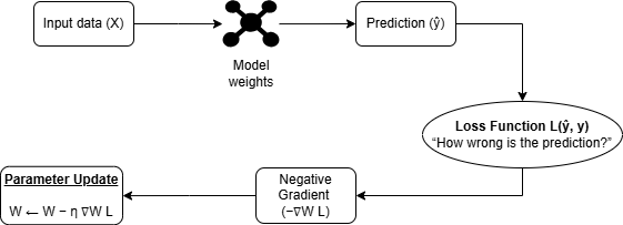
These are the steps you need to follow to apply the gradinet descent:
1- At the end of the forward pass, compute the loss:
How wrong the model is:
\[ L(W) \]
2- Compute the gradient:
Measures how much the loss changes with respect to each parameter, it tells us the direction and rate at which we should adjust each parameter to minimize the loss. \[ \frac{\partial L}{\partial W} \]
3- Update the parameters:
We update the model parameters (weights and biases) by moving them in the direction that reduces the loss. \[ W_{\text{new}} = W_{\text{old}} - \eta \frac{\partial L}{\partial W} \]
where \(\eta\) is the learning rate.
4- Keep repeating steps 2 → 4 until:
- Loss stops decreasing
- Or maximum iteraions reached
There are two types of gradient decent update, we apply the update after summing all losses from all data samples, using the full batch (Batch Gradient Decent), or the second method is to update the parameters after getting the loss of a single sample (Stochastic Gradient Descent (SGD)), here is a comparison table between the two:
Comparison Table: Batch Gradient Descent vs. Stochastic Gradient Descent
| Method | Loss Calculation | Gradient Calculation | Parameter Update Frequency |
|---|---|---|---|
| Batch Gradient Descent | \(L = \frac{1}{N} \sum_{i=1}^{N} L^{(i)}\) | \(\nabla L = \frac{1}{N} \sum_{i=1}^{N} \nabla L^{(i)}\) | Once per epoch (all samples) |
| Stochastic Gradient Descent (SGD) | \(L = L^{(i)}\) | \(\nabla L = \nabla L^{(i)}\) | After each sample |

Notice how the loss in SGD is dropping but with high randomness, while the Full bactch GD is dropping smoothly.
Momentum
In Momentum, the previous gradients are accumulated and added to each new update, this creates an inertia effect that accelerates the optimization process. It forces the update to move in the direction that consistently reduce the loss, because it is accumulating previous gradients, you can think of the process as if it remembers where it was going before and uses that memory to move more efficiently in the next step.
The mathematical update rule for Momentum is:
First, we take the accumulated gradients (velocity), \[ v_{t} = \beta v_{t-1} + \nabla L(w_{t}) \]
Where:
\(v_{t}\) is the velocity (accumulated gradient) at step \(t\)
\(\beta\) is the momentum coefficient (e.g., 0.9), it controls how much of the previous accumulated gradient (velocity) is retained in the current update.
\(\nabla L(W_{t})\) is the gradient at step \(t\).
Then the new weight update will be like this: \[ w_{t+1} = w_{t} - \eta v_{t} \]
By using this method, the model will not just update the weights based on the current calculated gradient, instead it combines all previous gradients (accumulates information) then use them in this new update. This accumulation creates a momentum effect, allowing the optimizer to maintain its direction and increase its speed. As a result, it helps the model converges faster.
Code
In each epoch, we calculate the gradiants grads = gradients(y_pred) then use it to create the velocity, which accumulates information from all previous gradients. The beta parameter controls how much we need to keep the previously calculated gradaints and use them for the next update. This allows the optimizer to build momentum and move more efficiently toward the minimum.
RMSProp
The RMSProp (Root Mean Square Propagation) algorithm was introduced to stablize the gradient descent update even more than what Momentum is doing. Before RMSProp, algorithms use one global learning rate for all parameters.
This causes problems:
Makes large updates for parameters with large gradients, where we should be more cautious.
Very small updates for parameters with small gradients, where we may want to explore further.
RMSProp overcome these issues by adapting the learning rate for each parameter individually, instead of using one global learning rate. It does this by:
1- Instead of remembering all past gradients, RMSProp only keeps the average of the squared gradients.
2- It does not update the gragient directly, insted it updates using the running average.
Math
Before, we updated the parameters directly: \[ \theta = \theta - \eta g_t \text{[direct update]} \]
In RMSProp, we need the running average, which tracks how large or small the gradients are for each parameter over time. If gradients large, then the learning rate will be smaller, thus applying smaller updates for the parmater, and the opposite is true. This helps stabilize training and prevents the learning rate from being too aggressive or too slow for different parameters.
The running avergage: \[ v_t = \beta v_{t-1} + (1 - \beta) g_t^2 \]
You could ask this: why using the squared gradient? The intuition behind this is that we care about the magnitude not the sign, the running average wants to find how large the gradients are, whiot caring about their sing.
Why use the squared gradient?
The intuition is that we care about the magnitude of the gradients, not their sign. By squaring the gradients, the running average finds how large the gradients are, regardless of direction. The update will be based on size only of recent gradients.
Then update the parameters using this: \[ W = W - \frac{\eta}{\sqrt{v_t + \epsilon}} g_t \]
where:
\(g_t\) is the current gradient,
\(v_t\) is the running average of squared gradients,
\(\eta\) is the learning rate,
\(\epsilon\) is a small constant to avoid division by zero.
Code
The difference in this code than what we did in Momentum is that we need to find the running average, velocity = beta * velocity + (1-beta) * grads**2, then rather than applying a fixed learning rate to all parameters, RMSProp divides the learning rate by the root of the running average. Larger gradients will get smaller learning rate, and smaller gradients will get larger learning rate updates, allowing for bigger updates.
Adam
Combining the advantages of both Momentum and RMSprop techniques, Adam optimizer achives the best results and is currently the most popular optimization algorithms used in deep learning. It stands for Adaptive Moment Estimation. It adapts the learning rate for each parameter (Like what we did in RMSprop), and applies the acceleration provided by momentum. With this, it often converges faster and more reliably than other optimizers.
Let’s look at how it works in details:
Math
Adam maintains two running averages, the first one \(m_t\) captures the average direction of recent gradients,and the second one is capturing the average magnitude of the gradients:
The first moment (captures the average direction): \[ m_t = \beta_1 m_{t-1} + (1 - \beta_1) g_t \]
The second moment (captures the average magnitude): \[ v_t = \beta_2 v_{t-1} + (1 - \beta_2) g_t^2 \]
Bias correction: We need to apply this because both \(\hat{m}_t\) and \(\hat{v}_t\) are initialized at zero, thus, and in order to prevent them from being biased towards zero during the initial training steps, the following corrections are used: \[ \hat{m}_t = \frac{m_t}{1 - \beta_1^t} \] \[ \hat{v}_t = \frac{v_t}{1 - \beta_2^t} \]
Parameter update: \[ W = W_{t-1} - \frac{\eta}{\sqrt{\hat{v}_t} + \epsilon} \hat{m}_t \]
where: - \(g_t\) is the gradient at time \(t\) - \(m_t\) is the first moment (mean) - \(v_t\) is the second moment (variance) - \(\beta_1, \beta_2\) are decay rates (e.g., 0.9 and 0.999) - \(\eta\) is the learning rate - \(\epsilon\) is a small constant for numerical stability
Code
In this code we will use the previously defined functions, so make sure to run the previous code cells. The code will show the difference between using a bias correction and without using it:
We can notice two things:
1- Blue curve (“WITHOUT bias correction”): The loss decreases slowly and remains much higher throughout training.
2- Orange curve (“WITH bias correction”): The loss decreases much faster and reaches a much lower value.
Bias correction is essential, and without it the optimizer will keep making smaller and less effective updates due to the underestimation of the magnitude and velocity caused by theri zero initialization in the early training step.
Summary
We covered the fundementals of the most popular optimization algorithms used in deep learning. Gradient decent is the basic parameter update method, and we saw the two types of GD: Batch Gradient Decent anf Stochastic Gradient Descent (SGD). Then introduced Momentum, which accelerate convergance by accumulating the moving average of past gradients helping smooth noisy updates. However, momentum alone does not account for the scale of the gradients, meaning parameters with large gradients can still receive overly large updates. RMSProp addresses this issue by maintaining a running average of squared gradients, allowing for adaptive learning rates for each parameter. Adam combines the benefits of both Momentum and RMSProp by keeping running averages of both the gradients and their squares, along with bias correction to ensure accurate estimates early in training.
Comments