Backward propagation in Convolutional Neural Networks (CNNs): Intuition, Math, and a Simple Example

In previous post we discussed the basics of a forward pass in a convolutional neural network (CNN). Now let’s dive into the backward pass, and see how the gradients are calculated and how the weights are updated during training.

We will discuss the following:

• Recap of Forward Pass

• Backward Pass

• Backward Pass Math

• Code & Example

Recap of Forward Pass

The forward pass in a CNN is applying a convolution operation between the input image and a filter (or kernel) to produce a feature map. Here is a simple example:

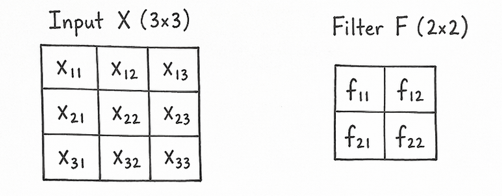
We have a 3x3 input image and a 2x2 filter. The convolution operation involves sliding the filter over the input image and performing element-wise multiplication and summation to produce the output feature map.

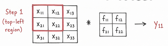
The above image shows a 3x3 input image convolved with a 2x2 filter, the math is as follows: \[ y_{11} = (x_{11}*f_{11}) + (x_{12}*f_{12}) + (x_{21}*f_{21}) + (x_{22}*f_{22}) \]

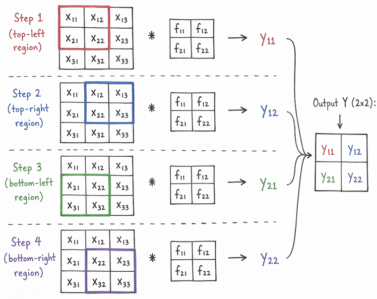
Then we redo the same process for the next position of the filter until we have covered the entire input image, resulting in a 2x2 output feature map.

Backward Pass

The backward pass is a process of calculating the gradients of the loss function with respect to the weights of the filters in the convolutional layer. This refers to how much each weight in the filter contributed to the final output, thus telling us how to adjust the weights to minimize the loss.

First let’s see how the loss is calculated. Here is the equation for categorical cross-entropy loss function: \[ \text{Loss} = -\frac{1}{n} \sum_{i=1}^{n} \sum_{c=1}^{C} y_{i,c} \log(\hat{y}_{i,c}) \]

For each training example, we calculate the predicted probabilities \(\hat{y}_{i,c}\) for each class \(c\) using the output of the CNN and the softmax function. Then we compare these predicted probabilities with the true labels \(y_{i,c}\) to compute the loss.

To start the backward pass, we need to compute the gradients of the loss with respect to the output \(Y\), given by: \[ \frac{\partial \text{L}}{\partial Y} = \begin{bmatrix} \frac{\partial L}{\partial y_{11}} & \frac{\partial L}{\partial y_{12}} \\ \frac{\partial L}{\partial y_{21}} & \frac{\partial L}{\partial y_{22}} \end{bmatrix} \]

Backward Pass Math

In the forward pass, we hade performed 3 computations:

1. conv(X, F) to get Y

2. softmax(Y) to get the predicted probabilities

3. loss(predicted probabilities, true labels) to get the loss

In the backward pass, we start from the loss and compute the gradients in reverse order:

1. Compute the gradient of the loss with respect to the predicted probabilities: \[ \frac{\partial \text{L}}{\partial Y} \]

2. Compute the gradient of \(Y\) with respect to the filter \(F\) : \[ \frac{\partial Y}{\partial F} = X \]

To see how we got the above equation, refer to the convolution operation: \[ y_{11} = (x_{11}*f_{11}) + (x_{12}*f_{12}) + (x_{21}*f_{21}) + (x_{22}*f_{22}) \]

The gradient of \(y_{11}\) with respect to \(f_{11}\) is: \[ \frac{\partial y_{11}}{\partial f_{11}} = x_{11} \]

3. Compute the gradient of the loss with respect to the filter \(F\) using the chain rule: \[ \frac{\partial L}{\partial F} = \frac{\partial L}{\partial Y} \cdot \frac{\partial Y}{\partial F} = \frac{\partial L}{\partial Y} \cdot X \]

4. Gradient with respect to the input image \(X\):

The forward pass for \(x_{11}\) is: \[ y_{11} = (x_{11}*f_{11}) + (x_{12}*f_{12}) + (x_{21}*f_{21}) + (x_{22}*f_{22}) \]

We can see that \(x_{11}\) contributes to only one output \(y_{11}\).

Take \(\frac{\partial L}{\partial x_{11}}\) as an example, we can compute it as follows: \[ \frac{\partial L}{\partial x_{11}} = \frac{\partial L}{\partial y_{11}} \cdot \frac{\partial y_{11}}{\partial x_{11}} = \frac{\partial L}{\partial y_{11}} \cdot f_{11} \]

Again do the same for \(x_{21}\), starting from the forward pass: \[ y_{11} = (x_{11}*f_{11}) + (x_{12}*f_{12}) + (x_{21}*f_{21}) + (x_{22}*f_{22}) \]

\[ y_{21} = (x_{21}*f_{11}) + (x_{22}*f_{12}) + (x_{31}*f_{21}) + (x_{32}*f_{22}) \]

We can see that \(x_{21}\) contributes to both \(y_{11}\) and \(y_{21}\), so we need to sum the contributions from both outputs: \[ \frac{\partial L}{\partial x_{21}} = \frac{\partial L}{\partial y_{11}} \cdot \frac{\partial y_{11}}{\partial x_{21}} + \frac{\partial L}{\partial y_{21}} \cdot \frac{\partial y_{21}}{\partial x_{21}} = \frac{\partial L}{\partial y_{11}} \cdot f_{21} + \frac{\partial L}{\partial y_{21}} \cdot f_{11} \]

The process is similar for the other input pixels, we need to pay attention to which output pixels they contribute to and sum the contributions accordingly. The middle pixle \(x_{22}\) contributes to all four output pixels, so its gradient will be the sum of contributions from all four outputs:

\[ \frac{\partial L}{\partial x_{22}} = \frac{\partial L}{\partial y_{11}} \cdot f_{22} + \frac{\partial L}{\partial y_{12}} \cdot f_{12} + \frac{\partial L}{\partial y_{21}} \cdot f_{12} + \frac{\partial L}{\partial y_{22}} \cdot f_{11} \]

In backward pass, we ask: “which output pixels does this input pixel contribute to?”

Some pixles contribute to only one output pixel, and others to multiple output pixels. So, the \(\frac{\partial L}{\partial x}\) is another convolution operation between the output gradients \(\frac{\partial L}{\partial Y}\) and the filter \(F\). See this pattern:

$$ \[\begin{aligned} \frac{\partial L}{\partial x_{11}} &= dy_{11} \cdot f_{11} \\ \frac{\partial L}{\partial x_{12}} &= dy_{11} \cdot f_{12} + dy_{12} \cdot f_{11} \\ \frac{\partial L}{\partial x_{13}} &= dy_{12} \cdot f_{12} \\ \\ \frac{\partial L}{\partial x_{21}} &= dy_{11} \cdot f_{21} + dy_{21} \cdot f_{11} \\ \frac{\partial L}{\partial x_{22}} &= dy_{11} \cdot f_{22} + dy_{12} \cdot f_{21} + dy_{21} \cdot f_{12} + dy_{22} \cdot f_{11} \\ \frac{\partial L}{\partial x_{23}} &= dy_{12} \cdot f_{22} + dy_{22} \cdot f_{12} \\ \\ \frac{\partial L}{\partial x_{31}} &= dy_{21} \cdot f_{21} \\ \frac{\partial L}{\partial x_{32}} &= dy_{21} \cdot f_{22} + dy_{22} \cdot f_{21} \\ \frac{\partial L}{\partial x_{33}} &= dy_{22} \cdot f_{22} \end{aligned}\]

$$

The pattern is applying a convolution operation between the output gradients \(\frac{\partial L}{\partial Y}\) and the filter \(F\) rotated by 180 degrees.

Code & Example

Note

Refer to this simple training process: cnn_with_pytorch.ipynb